

Forced Convection of a Non-Newtonian Nanofluid in Tube, Paper Numerical Validation
Price: $54
This simulation is based on the information of a reference article "Modeling of forced convective heat transfer of a non-Newtonian nanofluid in the horizontal tube under constant heat flux with computational fluid dynamics" and its results are compared and validated with the results in the article.
Paper Description
The present problem simulates the forced heat transfer of a non-Newtonian nanofluid in a horizontal tube using ANSYS Fluent software. This simulation is based on the information of a reference article "Modeling of forced convective heat transfer of a non-Newtonian nanofluid in the horizontal tube under constant heat flux with computational fluid dynamics" and its results are compared and validated with the results in the article. The nanofluid used in this model consists of water as the base fluid and xanthan and Al2O3 particles as its nano particles. The presence of xanthan causes the fluid to become non-Newtonian, and the presence of aluminum oxide particles causes the base fluid to become nanofluid.
The multiphase flow model is not used to define the nanofluid in this model; Rather, it is defined as a new material with thermophysical properties related to a nanofluid. Therefore, the current nanofluid inside the tube is defined with a density equal to 1126.384 kg.m-3 and a specific heat capacity equal to 3700.264 j.kg-1.K-1 and a thermal conductivity equal to 0.615 Wm-1.K-1. Be. Each of the values of the above thermophysical properties is obtained according to the relationships in the mentioned article. As mentioned, this nanofluid is a non-Newtonian fluid; So, it does not follow Newton's law of fluids, and its viscosity changes with force.
Paper Description
Therefore, considering that the nanofluid flowing in the tube is a non-Newtonian fluid, the viscosity of the nanofluid is defined based on the herschel-bulkley model. According to the herschel-bulkley relationship, the values of the power-law coefficient and the yield stress threshold and the critical stress rate are 0.149, 2.92 pascal and 58.4 1.s-1, respectively. These coefficients are defined based on the data in Table 1 of the article. In this simulation, the nanofluid concentration is 4% and the nanofluid flow has two different Reynolds values (900 and 1600).
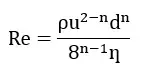
The following equation represents the value of the Reynolds number in terms of the value of the flow velocity in a non-Newtonian flow, the value of ƞ being defined in Table 1 of paper. So the value of the inlet flow velocity of the pipe is obtained according to this relation. This non-Newtonian nanofluid flows into the tube at a temperature of 295 K; So that the tube under constant heat flux is equal to 8846.4 W.m-2.
Geometry & Mesh
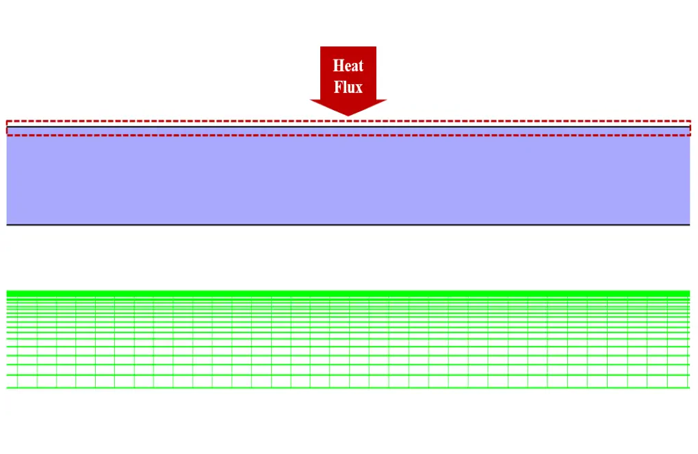
The present model is designed in two dimensions using Design Modeler software. This model includes a two-dimensional horizontal tube with a length of 1.2 m and a diameter of 0.00475 m. Since this model has a symmetric geometric, it is drawn as axisymmetric with cylindrical coordinates.
We carry out the meshing of the model using ANSYS Meshing software, and the mesh type is structured. The element number is 40000. The following figure shows the mesh.
Forced Convection CFD Simulation
We consider several assumptions to simulate the present model:
- We perform a pressure-based solver.
- The simulation is steady.
- The gravity effect on the fluid is ignored.
The following table represents a summary of the defining steps of the problem and its solution:
| Models (Forced Convection) | ||
| Viscous | Laminar | |
| Energy | On | |
| Boundary conditions (Forced Convection) | ||
| Inlet | Velocity Inlet | |
| velocity magnitude | 1.732714752 or 1.269787769 m.s-1 | |
| temperature | 295 K | |
| Outlet | Pressure Outlet | |
| gauge pressure | 0 pascal | |
| wall motion | stationary wall | |
| heat flux | 8846.4 W.m-2 | |
| Axis | Axis | |
| Methods (Forced Convection) | ||
| Pressure-Velocity Coupling | SIMPLE | |
| pressure | second order | |
| momentum | second order upwind | |
| energy | second order upwind | |
| Initialization (Forced Convection) | ||
| Initialization methods | Standard | |
| gauge pressure | 0 pascal | |
| axis-velocity | 1.732715 or 1.269788 m.s-1 | |
| temperature | 295 K | |
Paper Validation & Results of Forced Convection
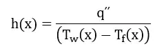
The validation of the present simulation is based on the diagram in Figure 3-a of the mentioned article. This graph is related to the changes in the heat transfer coefficient of model (h) relative to the changes in the Reynolds number value. This diagram is for a state for which a dimensionless parameter defined in x/D form is equal to 147; So that parameter D indicates the size of the model diameter, which is equal to 0.00475 m. We perform the present simulation in two different values for the Reynolds number of 900 and 1600. The value of heat transfer coefficient is obtained according to the following equation (equation number 9 of the article).
Paper Validation & Results of Forced Convection
The amount of heat flux in this regard according to the data of the article is equal to 8846.4 W.m-2. Also Tw represents the wall temperature of the model and Tf represents the bulk temperature of the fluid. To obtain the value of these temperatures, we must create the resulting x value in the location (according to the above), a point on the model wall and a line passing through the model, respectively, and then we can obtain the values of the temperatures on them.
| Error (%) | present simulation | paper simulation | |
| 0.014 | 1676.1 | 1700 | heat transfer coefficient (W.m-2.K-1) @ Re = 900 |
| 0.055 | 1846.8 | 1750 | heat transfer coefficient (W.m-2.K-1) @ Re = 1600 |
At the end of the solution process, we obtain two-dimensional temperature and velocity counters in two different Reynolds values (900 and 1600). These contours are correspond to the middle part of the model.