

Heller Dry Cooling Tower CFD Simulation
Price: $20
In this project, the airflow inside a dry cooling tower (HELLER) is simulated and analyzed by ANSYS Fluent.
Heller Dry Cooling Tower CFD Simulation
Price: $20
In this project, the airflow inside a dry cooling tower (HELLER) is simulated and analyzed by ANSYS Fluent.

Heller Dry Cooling Tower CFD Simulation, ANSYS Fluent Training
A dry cooling tower is used as a means of indirect heat transfer between the working fluid (water) and the coolant(air). In a thermal plant, the working fluid (water) exits the condensers and then is pumped into a ring of heat exchangers. These heat exchangers are air-cooled, which means that they are cooled by natural air suction caused by a temperature difference between the inside and the outside of the cooling tower.
The more the temperature difference exists between outside air and working fluid, the stronger the temperature driving force. In the summer, the temperature difference between the working fluid and the ambient air decreases, which will result in a reduction in temperature driving force, making the cooling tower’s efficiency to decrease.
Therefore, the thermal unit has to lower its power production, and the rate of water consumption will increase drastically to cool the heat exchangers. In this project, the airflow inside a dry cooling tower (HELLER) is simulated and analyzed by ANSYS Fluent.
Heller Geometry & Mesh
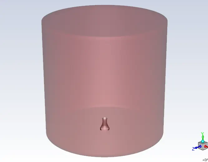
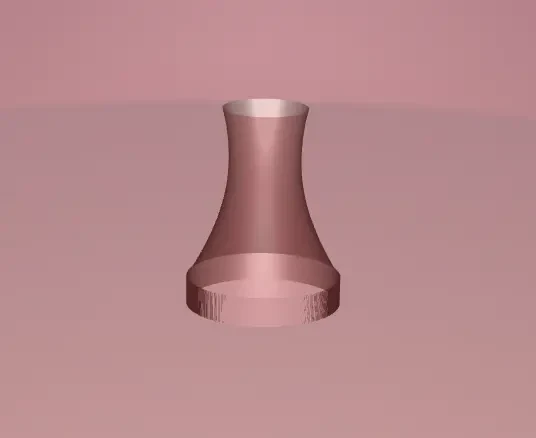
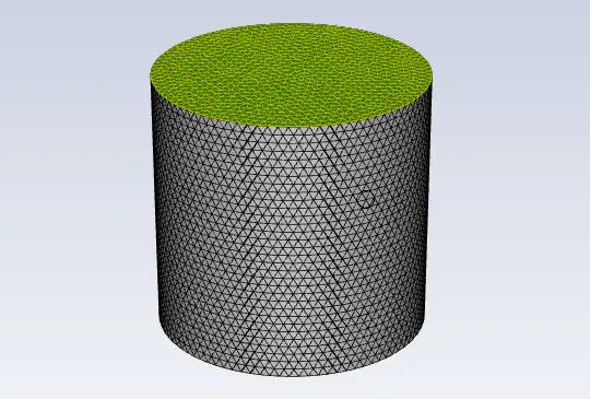
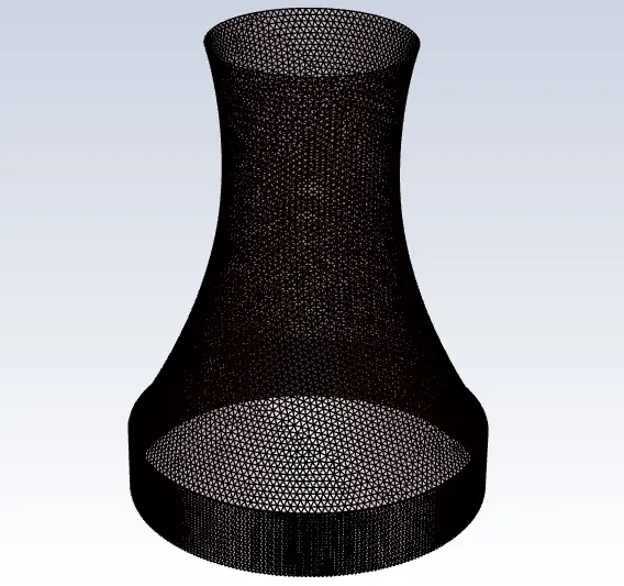
The geometry of this project includes a cooling tower, heat exchanger, flow domain, and an air inlet. The geometry is designed and meshed inside GAMBIT. The mesh type used for this geometry is unstructured and the total element number is 1343988 cells.
CFD simulation
The assumptions considered in this project are:
- Simulation is done using a pressure-based solver.
- The present simulation and its results are considered to be steady and do not change as a function time.
- The effect of gravity has been taken into account and is equal to -9.81m/s2 in the Y direction.
The applied settings are recapitulated in the following table.
| (Heller) | Models | |
| Viscous model | k-epsilon | |
| k-epsilon model | standard | |
| near-wall treatment | standard wall function | |
| Energy | on | |
| (Heller) | Boundary conditions | |
| Inlet | Pressure inlet | |
| Gauge total pressure | 0 Pa | |
| Direction specification method | Normal to boundary | |
| Outlet | Pressure outlet | |
| Gauge pressure | 0 Pa | |
| Backflow direction specification method | Normal to boundary | |
| temperature | 303 K | |
| Walls | ||
| Heller, Heller shadow | wall motion | stationary wall |
| Wall, wall shadow | heat flux | 0 W/m-2 |
| wall motion | stationary wall | |
| Radiator | Temperature | 318 K |
| Heat generation rate | 14861.52 W/m3 | |
| wall motion | stationary wall | |
| Radiator shadow | Temperature | 313 K |
| Heat generation rate | 14861.52 W/m3 | |
| (Heller) | Solution Methods | |
| Pressure-velocity coupling | SIMPLE | |
| Spatial discretization | pressure | standard |
| density | first-order upwind | |
| momentum | first-order upwind | |
| energy | first-order upwind | |
| turbulent kinetic energy | first-order upwind | |
| turbulent dissipation rate | first-order upwind | |
| (Heller) | Initialization | |
| Initialization method | Standard | |
| gauge pressure | 0 Pa | |
| velocity (x,y,z) | 0 m/s-1 | |
| temperature | 303.0806 K | |
| Turbulent kinetic energy | 1 m2/s2 | |
| Turbulent dissipation rate | 1 m2/s3 |
Heller Results
The contours of velocity, pressure, temperature, and flow streamlines are obtained at the end of the solution process.