
Build Your First Real Fluent Simulations
Price: $19
Ready to go beyond the fundamentals of ANSYS Fluent CFD? This intermediate bundle builds directly on Start Learning CFD Simulation by ANSYS Fluent, adding a second, more demanding project to every topic, multiphase flow, rotating machinery, dynamic mesh, combustion, radiation, FSI and more, across 16+ engineering fields. Backed by AI-assisted guidance, HPC computing power, and our internship pathway.
UDF: Pulsatile Blood Flow in Arterial Bifurcation
Project OverviewThis project presents an ANSYS Fluent simulation of time-dependent pulsatile blood flow through a simplified arterial bifurcation model.Geometry and MeshingThe fluid domain was created in Design Modeler, with mesh generation performed in ANSYS Meshing. An unstructured mesh containing 168,367 elements was employed for the computational domain.Boundary ConditionsBlood mass flow rates are specified as 0.001570178 kg/s at the inlet and 0.00078576 kg/s at each outlet. Inlet blood pressure is set at 250 Pa (approximately 1.87515 mmHg). For reference, physiological blood pressure in major human arteries typically ranges between 80 and 120 mmHg.Pulsatile Flow ImplementationThe pulsatile characteristics of blood flow are captured through a User-Defined Function (UDF), which modulates inlet velocity as a sinusoidal function of time, replicating the cardiac cycle’s rhythmic nature.Results and Clinical InsightsThe transient solver provides time-resolved flow data, with results presented at t = 0.162s, corresponding to peak systolic velocity. The simulation yields clinically relevant insights into arterial pathology susceptibility.High-Pressure Risk Zones: Pressure contour analysis at t = 0.16s reveals critical stress concentrations at the bifurcation apex, where flow streams diverge. Blood pressure reaches 125 Pa at this location—approximately half the inlet pressure—identifying this region as vulnerable to arterial wall rupture.Stenosis-Prone Regions: Wall Shear Stress (WSS) distribution analysis identifies areas susceptible to stenosis formation. Consistent with medical literature establishing low WSS as a stenosis predictor, the bifurcation apex exhibits minimal shear stress values, indicating heightened risk for atherosclerotic plaque development and subsequent arterial narrowing.
Build Your First Real Fluent Simulations
Price: $19
Ready to go beyond the fundamentals of ANSYS Fluent CFD? This intermediate bundle builds directly on Start Learning CFD Simulation by ANSYS Fluent, adding a second, more demanding project to every topic, multiphase flow, rotating machinery, dynamic mesh, combustion, radiation, FSI and more, across 16+ engineering fields. Backed by AI-assisted guidance, HPC computing power, and our internship pathway.
-
Section 1
Engineering Fields
$12-
The airfoil is the most fundamental geometry in all of aerodynamics — its shape governs the lift and drag that determine the performance of aircraft wings and turbine blades alike. In this project, you'll use ANSYS Fluent to study the airflow around a three-dimensional airfoil and learn to read the flow physics that engineers actually design around.You'll simulate an incompressible, isothermal airflow over a 0.5-meter NACA-type airfoil placed inside a wind tunnel domain, with a free-stream inlet velocity of 10 m/s. The mesh, built in ANSYS Meshing, is refined around the leading edge, the upper and lower surfaces, and the trailing edge to capture the boundary layer and wake accurately, while coarsening toward the far-field boundaries to keep the cell count efficient. The case is solved with a pressure-based, steady-state solver using the k–ω SST turbulence model.From the results, you'll learn to interpret the high-pressure stagnation region at the leading edge, the low-pressure suction zone on the upper surface that generates lift, and the pressure differential between the upper and lower surfaces that produces the net upward aerodynamic force. You'll also see how the velocity field accelerates over the suction side and develops a velocity deficit in the wake, where vortical structures and energy loss give rise to aerodynamic drag. Finally, you'll connect these flow features to the lift and drag coefficients and see why near-wall mesh refinement is essential for reliable predictions.By the end of this project, you'll be able to set up, solve, and analyze a complete external aerodynamics case in ANSYS Fluent — and understand the forces and losses behind the results, not just the contours.
Lesson 1 22m 7s -
When water spills over an ogee overflow and discharges into a pond, the way it behaves depends heavily on whether the flow runs as a free surface or under pressure. Capturing that difference is essential for designing spillways and overflow structures that handle their intended flow safely. In this project, you'll use ANSYS Fluent to simulate water flowing over an ogee spillway into a pond, comparing two distinct flow regimes side by side.The model is built in two dimensions in ANSYS DesignModeler as an ogee overflow leading into a pond, and two separate cases are studied. In the first, the flow is a free surface reaching the overflow at a defined height with a flow rate of 140 kg/s; in the second, the water flows under pressure with a flow rate of 420 kg/s. The geometry is also configured in two variants — one that includes an upstream region before the overflow and one that omits it — and the inlet is split into separate water-flow and airflow sections. Meshing is carried out in ANSYS Meshing using a semi-structured grid, with roughly 20,100 elements for the free-flow case and 16,400 for the pressure-flow case.Because both cases involve a moving interface between air and water, a two-phase Volume of Fluid (VOF) model is used, with air defined as the primary phase and water as the secondary phase. From the results, you'll examine 2-D contours of pressure and velocity along with the volume-fraction field that reveals the free surface and the path of the water into the pond. You'll also obtain a plot of static pressure along the flow direction for both models, allowing a direct comparison between the free-surface and pressurized regimes.By the end of this project, you'll be able to set up a two-phase free-surface flow in ANSYS Fluent using the VOF model, configure and compare multiple flow scenarios on a single hydraulic structure, and interpret the results to understand how overflow conditions change pressure and velocity behavior.
Lesson 2 12m 23s -
DescriptionThis project models internal airflow in a building atrium using ANSYS Fluent. Atriums—rooted in Roman architecture and now often multi-story with glazed roofs—provide daylight and ventilation for interior spaces. In this case, a cylindrical central atrium admits air at 2 m/s and 101,325 Pa through a lower inlet, with exhaust through an upper outlet.MethodologyThe 3D geometry of the complex and its cylindrical atrium is built in SpaceClaim. Meshing is performed in ANSYS Meshing with an unstructured grid of ~2,500,000 elements, locally refined near interior boundaries to better capture gradients.ConclusionThe simulation examines pressure and velocity distributions and overall airflow behavior within the atrium. Outputs include 2D/3D contours of pressure and velocity, plus pathlines and velocity vectors, enabling identification of zones with favorable comfort conditions.
Lesson 3 15m 30s -
When plaque builds up inside an artery, the narrowing of the vessel changes the way blood flows and, critically, the pressure it must overcome to pass through. Understanding that pressure behavior is central to diagnosing and treating cardiovascular disease, and CFD offers a powerful, non-invasive way to study it. In this project, you'll use ANSYS Fluent to simulate blood flow through a clogged artery and investigate how a blockage drives the pressure changes along the vessel.The model is a three-dimensional cylindrical vessel, 0.18 m long and 0.004 m in diameter, with a curved blockage at its center. The constriction is defined mathematically by a Gaussian function that describes how the vessel radius narrows along its length — here representing a 90% clogging severity with a defined slope through the blocked region — and is built in ANSYS DesignModeler by importing a set of coordinate points and revolving the resulting curve around the central axis. Blood is modeled as a fluid with a density of 1035 kg/m³ and a viscosity of 0.0043 Pa·s, entering at a mass flow rate of 0.013662 kg/s. The geometry is meshed in ANSYS Meshing with a structured grid of roughly 431,000 elements.The case is solved with a pressure-based, steady-state solver under the assumption of laminar flow, with gravity neglected. Blood enters through a mass-flow inlet, the outlet is set as a pressure outlet at zero gauge pressure, and the vessel wall is treated as a stationary no-slip wall. From the results, you'll examine 2-D and 3-D contours of pressure, velocity, and pressure gradient, along with a plot of static pressure measured along the dimensionless length of the vessel. The results show clearly that the largest pressure drop occurs as the blood squeezes through the clogged region.By the end of this project, you'll be able to build a parametric, function-defined biological geometry, set up a laminar internal-flow case in ANSYS Fluent, and interpret pressure and velocity fields to quantify how an arterial blockage affects blood flow.
Lesson 4 26m 38s -
A bubble trap is a deceptively simple device that solves an important problem in chemical and process engineering: removing unwanted gas bubbles from a liquid stream. It works purely on buoyancy — when bubble-laden fluid enters the trap, the chamber slows the flow down, and the gas, being far less dense than the liquid, rises and separates out so that clean liquid can leave from below. In this project, you'll use ANSYS Fluent to simulate that separation process and watch the trap do its job in real time.The model is built in two dimensions in SpaceClaim, with a mixture of water and bubbles entering through a side wall and a lower outlet that allows purified water to exit. The geometry is meshed in ANSYS Meshing with a total of roughly 32,000 cells. Because the device relies on the density difference between the two phases, the Volume of Fluid (VOF) multiphase model is used to track the air–water interface, and gravity is applied in the Y direction to drive the buoyant separation. A laminar model is used, and the simulation is run as unsteady so that the entire process of bubbles entering and being trapped can be observed as it develops.From the results, you'll follow the full sequence: the trap begins filled with water, the incoming mixture introduces bubbles, and the lighter gas phase rises to the surface where it escapes through the top outlet, while clean water leaves through the bottom — exactly the behavior a bubble trap is designed to produce. A transient animation captures this separation as it unfolds.By the end of this project, you'll be able to set up an unsteady two-phase VOF simulation in ANSYS Fluent, model buoyancy-driven phase separation, and interpret transient results to evaluate how effectively a gas–liquid separation device performs.
Lesson 5 17m 3s -
Eulerian: Carbonate Cake Filtration ANSYS Fluent TutorialDive into the intricate world of industrial filtration processes with our comprehensive tutorial on simulating carbonate cake filtration using ANSYS Fluent. This episode, part of our “Multi-Phase: All Levels” course, offers an in-depth exploration of the Eulerian multiphase model applied to a critical separation process.Understanding Carbonate Cake FiltrationFiltration is a fundamental process in many industries, crucial for separating solids from liquids. This tutorial delves into the complexities of carbonate cake filtration, providing insights into:The principles of physical separation in filtration processesFormation and impact of filter cakesChallenges in maintaining filter efficiencyIndustrial Applications and ImportanceDiscover how carbonate cake filtration is essential in various sectors:Water treatment and purificationChemical processing industriesEnvironmental remediation effortsSimulation Setup in ANSYS FluentFollow our detailed guide to set up a robust simulation of carbonate cake filtration:Geometry and Mesh GenerationLearn how to:Design the filtration unit geometry using ANSYS Design ModelerGenerate an appropriate structured mesh using ANSYS MeshingOptimize mesh quality for accurate results in complex multiphase scenariosEulerian Model ConfigurationMaster the setup of the Eulerian multiphase model to simulate the interaction between water, carbonate particles, and the carbon filter:Activating and configuring the Granular and Packed Bed sub-modelsSetting up phase property models for granular temperature calculationImplementing drag, lift, and virtual mass forces between phase pairsAdvanced Modeling TechniquesElevate your simulation skills with advanced techniques specific to filtration processes:Heat Transfer and Energy ModelingExplore the implementation of:Ranz-Marshall model for water-filter heat transferEnergy equation for temperature distribution calculationStandard k-epsilon model for turbulence modelingParticle Dynamics and Cake FormationLearn to accurately simulate:Particle-particle and particle-filter interactionsCake layer formation and growth over timeImpact of cake formation on filtration efficiencyResult Analysis and VisualizationDevelop skills in interpreting and visualizing complex multiphase simulation results:Analyzing carbonate concentration changes across the filterObserving temperature profiles in the feed waterUnderstanding the dynamics of cake layer formationApplications in Process OptimizationUnderstand the real-world impact of your simulations through:Case studies on filtration unit design optimizationExamples of how simulation results inform process efficiency improvementsDiscussions on scaling up filtration processes for industrial applicationsFuture Directions and Research OpportunitiesExplore potential areas for further research and development:Investigating the effects of different filter materials and structuresStudying the impact of particle size distribution on cake formationDeveloping predictive models for filter lifespan and maintenance schedulesBy completing this comprehensive tutorial, you’ll gain the skills to simulate complex carbonate cake filtration processes using ANSYS Fluent. Whether you’re a process engineer, CFD specialist, or a student in chemical engineering, this knowledge will empower you to contribute to cutting-edge developments in separation technologies and process optimization.Join us on this exciting journey into the world of advanced filtration technology and unlock new possibilities in enhancing industrial separation processes and filter designs!
Lesson 6 1h 2m 20s -
Mastering Microchannel Heat Transfer: Advanced CFD Simulation for Thermal EngineersWelcome to the “Microchannel Heat Source CFD Simulation” episode of our “THERMAL Engineers: INTERMEDIATE” course. This comprehensive module delves into the intricate world of microscale heat transfer, focusing on the application of Computational Fluid Dynamics (CFD) in analyzing and optimizing microchannel cooling systems using ANSYS Fluent. Immerse yourself in this cutting-edge aspect of thermal management and learn how to enhance cooling efficiency in compact electronic devices and high-performance computing systems through powerful CFD techniques.Understanding the Pre-configured Microchannel Heat Source ModelBefore diving into the simulation specifics, we’ll explore the fundamental concepts of microchannel heat transfer.Principles of Microscale Heat TransferDiscover the unique physics governing heat transfer at the microscale level and its implications for cooling system design.Key Components of a Microchannel Cooling SystemLearn about the critical elements that make up a microchannel heat sink and how they contribute to enhanced heat dissipation.Analyzing Fluid Flow and Heat Transfer in Microscale GeometriesThis section focuses on the complex fluid dynamics and thermal behavior within microchannel systems:Laminar Flow Characteristics in MicrochannelsGain insights into the flow regimes typical in microchannel geometries and their impact on heat transfer efficiency.Surface Area to Volume Ratio EffectsUnderstand how the high surface area to volume ratio in microchannels enhances heat transfer capabilities.Implementing Appropriate Boundary Conditions for Microchannel SimulationsDive into the specifics of setting up realistic simulation scenarios:Heat Source Definition and Thermal LoadsExplore how to define accurate heat generation conditions to simulate various electronic cooling scenarios.Fluid Inlet and Outlet ConditionsLearn to set appropriate flow rates, pressures, and temperatures for the cooling fluid in microchannel systems.Configuring ANSYS Fluent for Conjugate Heat Transfer in Small-Scale SystemsIn this section, we’ll guide you through the process of preparing your CFD simulation:Mesh Generation Strategies for Microchannel GeometriesMaster techniques for creating appropriate meshes that capture both fluid flow and solid heat conduction in microscale structures.Selecting Appropriate Physical Models for Microscale PhenomenaLearn to choose and configure the right models for accurate representation of heat transfer and fluid flow in microchannels.Investigating Temperature and Velocity Profiles Within MicrochannelsUnderstand how to analyze and interpret the key outputs of your simulation:Visualizing Fluid Flow Patterns in MicrochannelsDevelop skills in creating and interpreting velocity vector fields and streamlines to understand fluid behavior within the microchannel system.Analyzing Temperature Distributions in Solid and Fluid DomainsLearn to generate and interpret temperature contours to assess the cooling effectiveness of the microchannel design.Evaluating the Cooling Effectiveness of Microchannel DesignsThis section focuses on assessing the performance of microchannel cooling systems:Calculating Heat Transfer Coefficients and Nusselt NumbersDiscover methods for quantifying the heat transfer performance of microchannel systems under various conditions.Pressure Drop Analysis and Pumping Power RequirementsLearn to evaluate the hydraulic performance of microchannels and its impact on overall system efficiency.Interpreting Results to Understand Heat Dissipation in Microchannel SystemsMaster the art of translating CFD data into practical insights:Thermal Resistance Network AnalysisDevelop techniques for breaking down the thermal path and identifying bottlenecks in heat dissipation.Optimizing Microchannel Geometry for Enhanced CoolingLearn to use CFD results to fine-tune microchannel dimensions and layouts for improved thermal performance.Practical Applications and Industry RelevanceConnect simulation insights to real-world engineering challenges:Microchannel Cooling in High-Performance ElectronicsExplore how CFD simulations can inform the design of cooling solutions for advanced processors and power electronics.Scaling Microchannel Technology for Larger SystemsUnderstand how to apply microchannel cooling principles to larger-scale thermal management challenges in data centers and electric vehicles.Why This Module is Essential for Intermediate Thermal EngineersThis intermediate-level module offers a deep dive into advanced cooling technology CFD simulation, a critical skill in modern electronic thermal management. By completing this simulation, you’ll gain valuable insights into:Advanced principles of microscale heat transfer and fluid dynamicsIntermediate CFD techniques for modeling complex conjugate heat transfer scenariosPractical applications of CFD analysis in optimizing compact cooling solutionsBy the end of this episode, you’ll have developed essential skills in:Setting up and running comprehensive microchannel cooling simulations in ANSYS FluentInterpreting simulation results to assess cooling performance and identify potential improvementsApplying CFD insights to enhance thermal management in high-power density electronic systemsThis knowledge forms a crucial stepping stone for thermal engineers looking to specialize in advanced electronic cooling, providing a foundation for cutting-edge research in microfluidics, next-generation computing systems, and innovative thermal management solutions.Join us on this exciting journey into the world of microchannel heat transfer CFD simulation, and take your next steps towards becoming an expert in advanced thermal engineering for the electronics industry!
Lesson 7 11m 59s -
Computational Investigation of Liquid–Solid Two-Phase Flow in a Borehole: Implications for Gas and Petrochemical EngineeringThe interaction between flowing fluids and the surrounding formation within a borehole constitutes a fundamental concern in upstream hydrocarbon operations, where drilling provides the principal access to subsurface reservoirs. This study examines that interaction through a computational fluid dynamics (CFD) simulation of liquid–solid two-phase flow in a vertical wellbore, conducted in ANSYS Fluent. The objective is to characterise the mechanism by which soil grains detach from the borehole wall and become entrained in the fluid stream, a process of direct relevance to wellbore stability and solids production in oil and gas wells.An Eulerian multiphase formulation is employed, with water designated as the primary (continuous) phase and soil grains as the secondary (dispersed) phase. This approach is appropriate for particle-laden flows in which the volume fraction of the dispersed phase exceeds approximately ten percent, as is characteristic of the slurry-type regimes encountered in drilling and in petrochemical particulate processing. Turbulence is represented using the standard k–ε model with standard wall functions and a dispersed turbulence multiphase treatment, while the computational domain is reduced to a representative cylindrical sector to limit computational cost. Water enters the central region of the well at 1.6 m·s⁻¹ together with soil particles at 1 m·s⁻¹, and the unsteady, pressure-based solver resolves the evolving flow field and phase distribution.The results, presented as contours of phase volume fraction and velocity, indicate that a portion of the soil grains is liberated from the borehole wall and joins the fluid stream, while some fluid simultaneously penetrates the formation. This behaviour demonstrates that the shear stress generated at the fluid–solid interface exceeds the cohesive adhesion between soil grains — the governing condition for the onset of solids detachment.The findings carry several implications for gas and petrochemical engineering. First, the identification of the threshold at which interfacial shear overcomes grain cohesion provides a physical basis for predicting sand and solids production, a phenomenon responsible for erosion of downhole and surface equipment and for wellbore plugging. Second, the same fluid–formation interaction underlies wellbore stability: controlled flow preserves wall integrity, whereas excessive scouring promotes hole enlargement and instability. Third, the computed volume-fraction and velocity fields inform the assessment of drilling-fluid carrying capacity and cuttings transport, both central to effective hole cleaning. Collectively, the study offers quantitative insight into the conditions under which a formation begins to fail under imposed flow, thereby contributing to the design of safer wells and to improved strategies for solids control during drilling and completion.
Lesson 8 21m 54s -
Project OverviewIn this study, we conduct a comprehensive CFD analysis simulating the cooling process of an IGBT Heat Sink using ANSYS Fluent software. Our team has performed this computational fluid dynamics investigation to evaluate thermal management effectiveness.An insulated-gate bipolar transistor (IGBT) functions as a critical three-terminal power semiconductor component, commonly employed as an electronic switching device. These transistors generate considerable thermal energy during operation and can suffer performance degradation from excessive heat.Implementing cooling strategies such as air or liquid cooling mechanisms (particularly heat sinks) effectively dissipates this surplus heat, resulting in enhanced performance capabilities, significantly higher power densities, and more compact module designs.In our simulation setup, the heat sink interfaces with a heat source generating 14583 W/m² flux on one surface, while air circulates across the opposite surface at a 0.25 kg/s mass flow rate. This airflow serves as the primary cooling mechanism for the heat sink assembly.The simulation geometry comprises both the heat source and heat sink components. We designed and generated the mesh using Gambit® software, implementing an unstructured mesh configuration with 11,872,367 elements for detailed analysis.Analytical ApproachTo accurately model heat transfer dynamics, we activated the Energy Equation within the simulation. Additionally, we implemented the Laminar viscous model to properly resolve the airflow characteristics throughout the system.Results and FindingsOur analysis produced comprehensive visualization data including temperature distributions, velocity profiles, surface heat flux patterns, and Nusselt number representations. These contours clearly demonstrate how the cooler fluid flow effectively reduces the heat sink temperature.The thermal exchange between the cold fluid flow and the heat source successfully lowered the overall system temperature, confirming that the cooling mechanism meets the project's objectives. The simulation validates the effectiveness of the selected cooling approach for IGBT thermal management.
Lesson 9 19m 28s -
Mastering Cross Ventilation and Swamp Cooler Dynamics: Beginner's Guide to Thermal CFD SimulationWelcome to the “Cross Ventilation for Swamp Cooler Cooling CFD Simulation” episode of our “THERMAL Engineers: BEGINNER” course. This comprehensive module introduces you to the fascinating world of cooling heat transfer, focusing on the practical application of swamp cooler technology in room environments using ANSYS Fluent.Understanding Cross Ventilation Flow PatternsBefore diving into the simulation specifics, we’ll explore the fundamental concepts of cross ventilation and its role in cooling.Principles of Natural VentilationDiscover the basic principles governing natural ventilation and how they apply to indoor cooling strategies.Factors Influencing Cross Ventilation EfficiencyLearn about the key factors that affect cross ventilation performance, including building orientation, window placement, and external wind conditions.Simulating Temperature Distribution in Room EnvironmentsThis section focuses on the critical aspects of thermal modeling in indoor spaces:Heat Transfer Mechanisms in Indoor SpacesGain insights into the various heat transfer mechanisms at play in a room, including conduction, convection, and radiation.Thermal Comfort Parameters and Their SignificanceUnderstand the key parameters that define thermal comfort and how they are represented in CFD simulations.Evaluating Swamp Cooler PerformanceDive into the specifics of modeling and analyzing swamp cooler effectiveness:Swamp Cooler Working PrinciplesLearn about the fundamental principles behind evaporative cooling and how swamp coolers leverage these for indoor climate control.Key Performance Indicators for Cooling EffectivenessExplore the metrics used to assess the cooling performance of swamp coolers in different environmental conditions.Setting Up the Simulation EnvironmentIn this section, we’ll guide you through the process of preparing your CFD simulation:Geometry Preparation and Mesh GenerationMaster the basics of working with pre-designed room geometries and creating appropriate meshes for accurate results.Defining Material Properties and Boundary ConditionsLearn to set up realistic material properties and boundary conditions that accurately represent the cooling and ventilation scenario.Configuring Heat Transfer ModelsUnderstand the essential models required for simulating cooling processes:Selecting Appropriate Turbulence ModelsGain insights into choosing the right turbulence model for indoor airflow simulations.Implementing Energy Equations for Heat TransferLearn to activate and configure the energy equation to model heat transfer in your simulation.Analyzing Simulation ResultsDevelop skills in interpreting the outcomes of your CFD simulation:Visualizing Air Velocity ContoursMaster techniques for creating and interpreting air velocity contours to understand ventilation patterns.Interpreting Temperature Distribution MapsLearn to generate and analyze temperature distribution maps to assess cooling effectiveness throughout the room.Assessing Cooling EffectivenessLearn to evaluate the overall performance of your simulated cooling system:Calculating Cooling Efficiency MetricsDiscover methods for quantifying the cooling efficiency of your simulated swamp cooler system.Identifying Hot Spots and Stagnation ZonesDevelop skills in recognizing areas of ineffective cooling and propose improvements to the ventilation strategy.Practical Applications and Real-World RelevanceConnect simulation insights to tangible engineering challenges:Optimizing Room Layout for Enhanced CoolingExplore how CFD simulations can inform better room designs for optimal cooling performance.Energy Efficiency in Building Climate ControlUnderstand the role of CFD in developing energy-efficient cooling strategies for buildings.Why This Module is Essential for Beginner Thermal EngineersThis beginner-friendly module offers a practical introduction to thermal CFD simulation, focusing on the popular application of swamp cooler technology. By completing this simulation, you’ll gain valuable insights into:Basic principles of cross ventilation and evaporative coolingFundamental CFD techniques for modeling indoor thermal environmentsPractical applications of CFD in evaluating and optimizing cooling systemsBy the end of this episode, you’ll have developed essential skills in:Setting up and running basic thermal CFD simulations in ANSYS FluentInterpreting simulation results to assess cooling system performanceApplying CFD insights to improve indoor thermal management strategiesThis knowledge forms a crucial foundation for aspiring thermal engineers, providing a springboard for more advanced studies in HVAC system design, building energy efficiency, and thermal comfort optimization.Join us on this exciting journey into the world of thermal CFD simulation, and take your first steps towards becoming a proficient thermal engineer in the field of indoor climate control and energy-efficient building design!
Lesson 10 13m 53s -
Mastering River Hydraulics: Open Channel Two-Phase Flow in Rough Rivers CFD Simulation for BeginnersWelcome to the “Open Channel Two-Phase Flow in Rough Rivers CFD Simulation” episode of our “HYDRAULIC Engineers: BEGINNER” course. This comprehensive module introduces civil engineers to the complex world of river hydraulics using computational fluid dynamics (CFD). Learn how to leverage ANSYS Fluent to simulate and analyze open-channel flow in natural river systems, a crucial skill for effective water resource management and flood control.Understanding the Importance of Open-Channel Flow in River EngineeringBefore diving into the simulation specifics, let’s explore the fundamental concepts of open-channel flow and its significance in hydraulic engineering.The Role of Open-Channel Flow in Natural River SystemsDiscover how open-channel flow governs river behavior, influencing flood patterns, erosion processes, and overall water resource dynamics.Challenges in Modeling Rough River BedsLearn about the complexities involved in accurately representing natural river conditions, including bed roughness and its impact on flow characteristics.Introduction to ANSYS Fluent for River Flow AnalysisThis section focuses on familiarizing beginners with the ANSYS Fluent software environment:Navigating the ANSYS Fluent InterfaceGain insights into the basic layout and functionality of ANSYS Fluent, essential for efficient simulation setup and analysis of river systems.Understanding the CFD Workflow for Open-Channel SimulationsLearn the step-by-step process of setting up, running, and analyzing an open-channel flow CFD simulation in ANSYS Fluent.Setting Up a Basic Open-Channel Flow ModelMaster the art of creating a simple simulation environment for river hydraulics:Defining Geometry and Mesh for Open-Channel SimulationsLearn techniques for creating a basic geometry representing an open channel with a rough bed, along with appropriate meshing strategies for accurate flow analysis.Configuring Two-Phase Flow Properties in ANSYS FluentExplore methods for defining and implementing the properties of water and air in your open-channel flow simulation.Incorporating Rough Bed Conditions in Your ModelDive into the critical aspects of representing natural river beds in CFD simulations:Techniques for Modeling Bed RoughnessUnderstand different approaches to simulate bed roughness in ANSYS Fluent, including surface roughness parameters and geometric representations.Implementing Roughness Effects on Flow BehaviorLearn how to configure model settings to accurately capture the influence of bed roughness on water flow patterns and velocity profiles.Boundary Conditions for River Flow ScenariosMaster the setup of realistic boundary conditions for open-channel simulations:Specifying Inlet and Outlet ConditionsUnderstand how to set up appropriate inlet flow rates and outlet conditions that accurately represent various river flow scenarios.Implementing Free Surface and Wall Boundary ConditionsLearn to define proper boundary conditions for the water surface, channel walls, and bed to capture realistic open-channel flow behavior.Running Basic Simulations of Water Flow in Open ChannelsDevelop skills to execute and monitor your first open-channel CFD simulations:Setting Up Solver Parameters for Hydraulic SimulationsMaster the basics of configuring solver settings, including time-stepping and convergence criteria, suitable for open-channel flow simulations.Monitoring Simulation Progress and Ensuring StabilityLearn techniques for tracking simulation progress and identifying potential issues during the solving process.Analyzing Fundamental Flow Patterns and Velocity ProfilesDevelop expertise in extracting meaningful insights from your river flow simulations:Visualizing Water Flow Patterns in Open ChannelsMaster techniques for creating insightful visualizations of velocity fields and streamlines to understand flow behavior in rough river beds.Interpreting Velocity Profiles and Water Surface BehaviorLearn to analyze velocity distributions and water surface profiles, crucial for assessing river flow characteristics and potential flood scenarios.Introduction to Free Surface Modeling in River SystemsExplore the basics of capturing the water-air interface in your simulations:Understanding the Concept of Free Surface in Open-Channel FlowGain insights into how free surface modeling represents the dynamic interface between water and air in river systems.Basic Techniques for Visualizing Free Surface in River SimulationsLearn introductory methods for identifying and interpreting free surface behavior in your open-channel flow simulation results.Practical Applications and Civil Engineering RelevanceConnect simulation insights to real-world river engineering challenges:Applying CFD Insights to River Management and Flood ControlExplore how the flow patterns and velocity profiles observed in CFD simulations can inform river training works, flood prediction models, and erosion control strategies.Understanding the Limitations of Beginner-Level SimulationsGain awareness of the simplifications in this introductory course and the potential for more advanced analyses in future studies.Why This Module is Essential for Beginner Hydraulic EngineersThis beginner-level module offers an introduction to the powerful world of CFD in river engineering. By completing this simulation, you’ll gain valuable insights into:Basic application of ANSYS Fluent for simulating open-channel flow in rough riversEssential CFD techniques for capturing flow patterns and velocity profiles in natural channelsPractical applications of CFD analysis in river management and flood control engineeringBy the end of this episode, you’ll have developed foundational skills in:Setting up and running basic open-channel flow simulations using ANSYS FluentInterpreting simulation results to assess hydraulic characteristics of rough river bedsApplying CFD insights to enhance understanding of river behavior and inform water resource management decisionsThis knowledge forms a solid foundation for civil engineers looking to integrate advanced computational methods into their river engineering and hydraulic design toolkit, providing a springboard for more advanced studies in flood prediction, erosion control, and sustainable river management.Join us on this exciting journey into the world of open-channel CFD simulation, and take your first steps towards becoming a proficient hydraulic engineer equipped with cutting-edge computational tools for innovative river analysis and management!
Lesson 11 28m 50s -
What You'll BuildThis lesson walks you through a CFD simulation of a sea robot moving through water using the Dynamic Mesh technique — the essential method for problems where a body physically moves through the fluid domain and the computational cells must change shape and position over time.In this project, the robot (modeled as a cube) starts on one side of the domain and travels toward the inlet against an oncoming water stream, letting you study the pressure buildup ahead of it and the wake region trailing behind.What You'll LearnWhen and why a Dynamic Mesh is mandatory — whenever the location or shape of computational cells changes during the simulationHow smoothing and remeshing work together to maintain high-quality elements as the body moves, preventing the mesh degradation that causes solver errorsHow to configure remeshing intervals (here, every 50 iterations) to regenerate a fresh, high-quality meshHow to design a 2-D moving-body domain in Design Modeler and mesh it (~30,010 elements) in ANSYS MeshingWhy a transient solver is required for any Dynamic Mesh problemHow to impose a prescribed velocity profile on the moving body (3 m/s in the X-direction over 0–3 seconds)How to set up the surrounding flow with an inlet water velocity of 1.5 m/s using the standard k-ε turbulence modelHow to post-process velocity, pressure, turbulent viscosity contours, and streamlines — observing the elevated stagnation pressure ahead of the robot and the wake region behind itWhy It MattersDynamic Mesh is the gateway to simulating real motion — submarines, AUVs, valves, pistons, projectiles, and store separation. Mastering smoothing and remeshing here equips you for an entire class of moving-body CFD problems.
Lesson 12 14m 30s -
Master RBF Morph in ANSYS Fluent: Advanced Mesh Morphing TechniquesDive deep into the powerful world of design optimization with our comprehensive episode, “RBF Morph (Mesh Morphing) Concepts in ANSYS Fluent,” part of the acclaimed “RBF: All Levels” course. This essential lesson equips you with the knowledge and skills to leverage ANSYS Fluent’s advanced design optimization tools effectively.Episode Overview: Unlocking ANSYS Fluent's Design TabIn this detailed tutorial, you’ll gain an in-depth understanding of the design tab environment in ANSYS Fluent. We’ll guide you through each crucial step of the design optimization process, ensuring you grasp the rationale behind every option and feature.Key Learning ObjectivesNavigate the ANSYS Fluent design tab with confidenceUnderstand and apply gradient-based optimization techniquesMaster various morphing methods for mesh manipulationImplement and analyze adjoint solutions for sensitivity analysisComprehensive Exploration of Design Optimization Tools1. Design Tab Fundamentals- Thorough introduction to the design tab interface - Overview of key features and their significance in optimization workflows2. Gradient-Based Optimization Techniques- Deep dive into gradient-based methods - Understanding observables and operations crucial for effective optimization3. Advanced Design Tools and Morphing Methods- Exploration of various design tools available in ANSYS Fluent - Detailed look at different morphing methods and their applications4. Objective Setting and Constraint Management- Techniques for defining and modifying optimization objectives - Strategies for setting and managing design constraints effectively5. Gradient-Based Optimizer Mastery- In-depth analysis of the gradient-based optimizer - Tips and tricks for optimizing your design process6. Adjoint Solution Post-Processing- Advanced techniques in sensitivity analysis - Interpreting and applying adjoint solution results for design improvementsWhy This Episode Is EssentialProvides hands-on experience with ANSYS Fluent’s most powerful optimization toolsOffers practical insights for real-world design challengesEnhances your ability to create more efficient and effective designsPrepares you for advanced applications in subsequent course episodesWho Should WatchThis episode is ideal for:CFD engineers looking to enhance their optimization skillsMechanical and aerospace designers seeking advanced ANSYS Fluent knowledgeResearchers exploring cutting-edge design optimization techniquesAnyone involved in complex fluid dynamics simulations and design processesElevate Your Design Optimization ExpertiseDon’t miss this opportunity to master the intricacies of RBF Morph and Mesh Morphing in ANSYS Fluent. This episode is your gateway to becoming a proficient user of some of the most advanced design optimization tools available in the industry.What You'll GainProficiency in navigating and utilizing ANSYS Fluent’s design tabAdvanced knowledge of gradient-based optimization techniquesSkills to implement and analyze complex mesh morphing strategiesAbility to conduct sophisticated sensitivity analyses for design refinementEnroll now to transform your approach to CFD-based design optimization. Whether you’re optimizing aerodynamics, enhancing heat transfer systems, or refining complex fluid flow designs, this course will equip you with the tools and knowledge to excel in your field.Join us in exploring the cutting-edge of CFD technology and take your design optimization skills to the next level!
Lesson 13 1h 6m 30s -
Mastering Parabolic Solar Collector Design: Advanced CFD Simulation for Thermal EngineersWelcome to the “Parabolic Solar Collector CFD Simulation” episode of our “THERMAL Engineers: INTERMEDIATE” course. This comprehensive module delves into the world of advanced renewable energy systems, focusing on the application of Computational Fluid Dynamics (CFD) in analyzing and optimizing parabolic solar collectors using ANSYS Fluent. Immerse yourself in this innovative heat transfer technology and learn how to enhance thermal efficiency in solar energy applications through powerful CFD techniques.Understanding the Pre-configured Parabolic Solar Collector ModelBefore diving into the simulation specifics, we’ll explore the fundamental concepts of parabolic solar collectors.Principles of Concentrated Solar PowerDiscover the key design features that make parabolic solar collectors efficient in harnessing solar energy for various applications.Components of a Parabolic Solar Collector SystemLearn about the critical elements that comprise a parabolic solar collector, including the reflector, receiver tube, and working fluid.Analyzing Convective Heat Transfer Mechanisms in the CollectorThis section focuses on the complex heat transfer processes within parabolic solar collectors:Solar Radiation Absorption and Heat Flux DistributionGain insights into how solar energy is concentrated and absorbed along the receiver tube surface.Fluid-Wall Heat Transfer in the Receiver TubeUnderstand the convective heat transfer mechanisms between the heated tube wall and the working fluid.Implementing Appropriate Boundary Conditions for Fluid Flow and Heat TransferDive into the specifics of setting up realistic simulation scenarios:Solar Heat Flux and Thermal Radiation ModelingExplore how to define accurate heat flux conditions on the receiver tube surface based on solar concentration factors.Fluid Inlet and Outlet ConditionsLearn to set appropriate flow rates, temperatures, and pressures for the working fluid entering and exiting the collector.Configuring ANSYS Fluent for Thermal-Fluid SimulationsIn this section, we’ll guide you through the process of preparing your CFD simulation:Mesh Generation Strategies for Parabolic Collector GeometriesMaster techniques for creating appropriate meshes that capture both the complex parabolic reflector shape and the cylindrical receiver tube accurately.Selecting Appropriate Physical Models for Solar Thermal ApplicationsLearn to choose and configure the right turbulence, heat transfer, and radiation models for precise parabolic solar collector simulation.Investigating Temperature Distributions Along the Receiver TubeUnderstand how to analyze and interpret the key outputs of your simulation:Visualizing Temperature GradientsDevelop skills in creating and interpreting temperature contours to understand heat distribution along the receiver tube length.Analyzing Thermal Boundary Layer DevelopmentLearn to evaluate the thermal boundary layer characteristics and their influence on overall heat transfer efficiency.Evaluating Fluid Flow Patterns and Their Impact on Heat Transfer EfficiencyThis section focuses on assessing the fluid dynamics within the collector:Velocity Profile Analysis in the Receiver TubeDiscover methods for visualizing and interpreting fluid flow patterns to identify potential areas of improvement.Turbulence Effects on Heat TransferLearn to assess the impact of turbulent flow on enhancing convective heat transfer within the receiver tube.Interpreting Results to Optimize Collector Design for Maximum Thermal PerformanceMaster the art of translating CFD data into practical design improvements:Calculating Overall Thermal EfficiencyDevelop techniques for quantifying the collector’s performance under various operating conditions.Parametric Studies for Design OptimizationLearn to use CFD results to optimize key design parameters such as receiver tube diameter, reflector shape, and flow rates.Practical Applications and Industry RelevanceConnect simulation insights to real-world engineering challenges:Parabolic Trough Systems in Solar Power PlantsExplore how CFD simulations can inform the design and optimization of large-scale concentrated solar power installations.Integration with Thermal Energy Storage SystemsUnderstand how to apply CFD analysis to improve the efficiency of parabolic collectors coupled with thermal storage technologies.Why This Module is Essential for Intermediate Thermal EngineersThis intermediate-level module offers a deep dive into advanced renewable energy CFD simulation, a critical skill in modern solar thermal engineering. By completing this simulation, you’ll gain valuable insights into:Advanced principles of concentrated solar power and heat transfer in parabolic collectorsIntermediate CFD techniques for modeling complex geometries and multiphysics phenomenaPractical applications of CFD analysis in enhancing renewable energy system efficiencyBy the end of this episode, you’ll have developed essential skills in:Setting up and running comprehensive parabolic solar collector simulations in ANSYS FluentInterpreting simulation results to assess thermal performance and identify potential improvementsApplying CFD insights to enhance the efficiency of solar thermal systems and similar heat transfer devicesThis knowledge forms a crucial stepping stone for thermal engineers looking to specialize in renewable energy technologies, providing a foundation for advanced studies in solar thermal systems, energy efficiency, and innovative heat transfer solutions.Join us on this exciting journey into the world of parabolic solar collector CFD simulation, and take your next steps towards becoming an expert in advanced thermal engineering for sustainable energy applications!
Lesson 14 13m 29s -
Mastering Centrifugal Compressor Dynamics: Advanced CFD Simulation for Mechanical EngineersWelcome to the “Centrifugal Compressor CFD Simulation” episode of our “MECHANICAL Engineers: ADVANCED” course. This comprehensive module delves into the complex world of centrifugal compressor design and analysis, using ANSYS Fluent to explore the intricate aerodynamics within these critical turbomachinery components.Compressible Flow Modeling in Rotating MachineryBefore diving into the simulation specifics, we’ll explore the fundamental concepts of compressible flow modeling in the context of centrifugal compressors.Governing Equations for Compressible FlowsDiscover advanced techniques for implementing and solving the governing equations of compressible flow in ANSYS Fluent.Turbulence Modeling for High-Speed Rotating FlowsLearn to select and implement appropriate turbulence models for accurate simulation of high-speed flows in centrifugal compressors.Impeller and Diffuser Flow AnalysisThis section focuses on the critical aspects of flow behavior within the compressor’s key components:Impeller Passage Flow CharacteristicsMaster the process of simulating and analyzing complex flow patterns within the rotating impeller passages, including secondary flows and tip clearance effects.Diffuser Performance and Pressure RecoveryGain skills in investigating flow behavior and pressure recovery mechanisms within the compressor diffuser, both vaned and vaneless designs.Pressure Ratio and Efficiency CalculationsDive deep into the methods for assessing and optimizing compressor performance:Total-to-Total Pressure Ratio ComputationLearn to simulate and interpret the fundamental pressure ratio characteristics of centrifugal compressors across various operating conditions.Isentropic Efficiency Evaluation TechniquesExplore methods to compute compressor efficiency and develop strategies for performance optimization, considering both aerodynamic and thermodynamic aspects.Rotating Reference Frame ImplementationExamine the crucial aspects of modeling rotating machinery in CFD:Multiple Reference Frame (MRF) ApproachDevelop skills in implementing the MRF method for steady-state analysis of centrifugal compressors, including interface treatment between rotating and stationary domains.Sliding Mesh Technique for Transient AnalysisLearn techniques to set up and execute transient simulations using the sliding mesh approach for capturing time-dependent phenomena in compressor operation.Pressure and Temperature Distribution AnalysisIn this section, we’ll delve into the detailed thermodynamic field characteristics within the compressor:3D Pressure Field Visualization TechniquesMaster the process of visualizing and interpreting complex 3D pressure fields in centrifugal compressors using ANSYS Fluent, including shock wave identification in transonic designs.Temperature Contour Analysis for Performance EvaluationDevelop methods to analyze temperature distributions and their influence on compressor performance, efficiency, and material considerations.Impact of Rotational Speed on Compressor PerformanceExplore the critical relationship between impeller speed and compressor characteristics:Compressor Map Generation and AnalysisLearn to generate and interpret compressor maps, including surge and choke limits, for various rotational speeds.Mach Number Effects on Flow BehaviorDiscover techniques to simulate and analyze compressor behavior under subsonic, transonic, and supersonic flow regimes at different operating speeds.Velocity Profiles and Secondary FlowsExamine the intricate flow structures within the compressor:Blade-to-Blade Flow VisualizationExplore methods for visualizing and analyzing flow patterns on blade-to-blade surfaces, including potential flow separation and wake formation.Tip Clearance Flow AnalysisLearn to simulate and quantify the effects of tip clearance flows on compressor performance and efficiency.Practical Applications and Industry RelevanceConnect simulation insights to real-world engineering challenges:Aerospace Propulsion System DesignExplore how centrifugal compressor CFD simulations contribute to the design and optimization of aircraft engines and auxiliary power units.Industrial Process Compressor OptimizationDiscover the relevance of this technology in enhancing the performance of compressors used in various industrial processes, including oil and gas, petrochemical, and refrigeration applications.Advanced Result Interpretation and Performance AnalysisElevate your CFD skills with sophisticated data analysis techniques:Surge Margin Prediction and Stability AnalysisLearn to predict surge margins and analyze compressor stability using CFD results, crucial for safe and efficient operation.Parametric Studies for Design OptimizationDevelop strategies to conduct parametric studies for optimizing impeller and diffuser geometries to enhance overall compressor performance across the operating range.Why This Module is Essential for Advanced Mechanical EngineersThis advanced module offers a deep dive into the sophisticated world of centrifugal compressor dynamics using ANSYS Fluent. By mastering this simulation, you’ll gain invaluable insights into:Advanced CFD techniques for modeling complex compressible flows in high-speed rotating machineryThe intricate relationships between compressor geometry, operating conditions, and performance characteristicsPractical applications of CFD in aerospace, turbomachinery, and industrial process equipment designBy the end of this episode, you’ll have enhanced your skills in:Modeling and analyzing advanced centrifugal compressor scenarios in ANSYS FluentInterpreting complex CFD results to optimize compressor designs for various industrial and aerospace applicationsApplying cutting-edge fluid dynamics concepts to real-world engineering challenges in turbomachineryThis knowledge will elevate your capabilities as a mechanical engineer, enabling you to contribute to innovative solutions in fields where understanding and optimizing centrifugal compressor performance is critical.Join us on this advanced journey into the world of centrifugal compressor CFD simulation with ANSYS Fluent, and position yourself at the forefront of mechanical engineering technology in turbomachinery design and optimization!
Lesson 15 18m 49s -
Computational Simulation of Carbon Dioxide Dispersion in an Urban Street Canyon: Implications for Urban Planning EngineeringThe dispersion of vehicular emissions within densely built environments represents a central concern of contemporary urban planning, particularly in developing regions where air quality continues to deteriorate despite advances in emission-control technology. This study addresses that concern through a computational fluid dynamics (CFD) simulation of carbon dioxide transport along an urban street, performed in ANSYS Fluent. The objective is to quantify the extent to which free airflow disperses the CO₂ generated by vehicular exhaust within a representative city block, thereby providing a physically grounded basis for evaluating urban ventilation.The model is three dimensional and reproduces a configuration of building blocks bordering a city street, enclosed within a rectangular computational domain measuring 9 m × 13 m × 4 m. A continuous source region of 0.1 m height is defined along the street to represent the integrated production of carbon dioxide from traffic, with a generation rate of 4 kg·m⁻³. Free airflow enters through three lateral faces of the domain at a velocity of 0.2 m·s⁻¹ and a temperature of 300 K. Because two gaseous constituents — air and CO₂ — are considered, the Species Transport model is employed, solving a separate transport equation for each component of the mixture; the energy equation is activated to account for thermal effects. Turbulence is represented using the standard k–ε model with standard wall functions, and the governing equations are advanced using a transient, pressure-based solver, consistent with the aim of resolving the temporal evolution of pollutant concentration. The domain is discretised with an unstructured mesh of approximately 4.14 million elements, refined in the vicinity of the internal boundaries to enhance resolution where concentration gradients are steepest.The solution yields two- and three-dimensional contours of pressure, temperature, velocity, and the mass fractions of air and carbon dioxide throughout the domain, with particular attention to the region surrounding the source term. These fields characterise how the imposed airflow transports and dilutes the emitted CO₂ across the street canyon and around the surrounding structures.The findings bear directly on several aspects of urban planning engineering. First, the predicted distribution of pollutant mass fraction reveals zones of accumulation and stagnation, information that supports the siting of pedestrian areas, building entrances, and ground-level activities away from regions of elevated concentration. Second, the dependence of dispersion on the prevailing wind field underscores the role of street orientation, building height, and block spacing in promoting or impeding natural ventilation — design variables over which the planner exercises control. Third, the methodology provides a transferable framework for assessing the air-quality consequences of proposed developments prior to construction, enabling the evaluation of alternative urban geometries with respect to their capacity to disperse traffic-derived emissions. Collectively, the study demonstrates how CFD-based species transport modelling can inform the design of healthier and better-ventilated urban environments.
Lesson 16 17m 21s
-
-
Section 2
Flow Models
$6-
This project simulates the explosion of oil storage tanks and the subsequent dispersion of combustion pollutants across an urban area using ANSYS Fluent. The core of the analysis lies in modelling reacting flow: an explosion is fundamentally a rapid, energetic chemical reaction that consumes fuel and releases heat together with a range of gaseous products, and capturing that behaviour requires a flow model capable of tracking multiple chemical species and their transport through the surrounding air.The motivation is a real safety concern. In regions that host oil reservoirs, the tanks represent a persistent explosion hazard, and a single event can release large quantities of pollutants such as carbon dioxide and other combustion gases into the atmosphere. Where residential neighbourhoods and industrial units sit close to the tank farm, the way these pollutants spread and reach the surrounding population becomes a critical question for risk assessment and emergency planning. This simulation is built to answer exactly that question.The geometry is a three-dimensional urban domain measuring 6.6 km in length, 4.6 km in width and 200 m in height, created in Design Modeler. Within it, a dedicated zone contains eighteen cylindrical oil tanks, while several further zones represent residential and industrial districts. The domain is discretised with an unstructured mesh of 1,746,979 elements.Because the explosion involves extensive chemical reactions among several gaseous constituents, the Species Transport model forms the heart of the setup. Seven species are modelled — CO₂, SO₂, NO₂, CO, H₂O, C and air — with air acting as the background fluid throughout the domain. The effect of the explosion is introduced within the tank region through defined energy and mass sources: a heat source of 139,072.7 W/m together with production rates for each pollutant (for example, CO₂ at 0.1358 kg/m³·s, H₂O at 0.0679 kg/m³·s, CO at 0.0047 kg/m³·s, SO₂ at 0.000131 kg/m³·s, C at 0.0068 kg/m³·s and a very small NO₂ contribution). This source-based representation lets the model release the heat and combustion products of the explosion directly into the reacting-flow field.Wind is the primary driver of dispersion. The northern and western faces of the domain are set as airflow inlets and the eastern and southern faces as outlets. Open airflow enters at 300 K and 20 m/s, directed at 60° (with x- and y-velocity components of 20·cos60° and 20·sin60° respectively), so that wind speed and direction govern how far and in which direction the pollutant plume travels across the city.The solution yields three-dimensional contours of temperature and of the volume fraction of each gaseous species throughout the domain. The results demonstrate that, in the event of such an explosion, the released pollutants are carried into the surrounding residential and industrial zones, confirming the potential exposure of the urban population. As a study in chemical-reaction flow modelling, the project shows how species transport combined with defined energy and mass sources can reproduce the generation and atmospheric spread of combustion products — a powerful basis for evaluating explosion hazards and informing the siting, spacing and protection of facilities near populated areas.
Lesson 1 26m 39s -
This project simulates the flow over a NACA 0012 airfoil using ANSYS Fluent, with compressible flow as the central modelling theme. At the freestream conditions studied here, the air can no longer be treated as incompressible — density varies appreciably with pressure and temperature across the flow field — so the simulation is built around a compressible-flow formulation, making it a clear illustration of how that class of flow model is set up and solved.The airfoil is the cross-sectional shape of a lifting surface such as an aircraft wing, a wind-turbine blade or a helicopter rotor. The aerodynamic behaviour of a given design depends strongly on its profile, which is why different airfoils are selected for different applications. The geometry is defined by familiar parameters: the chord line, the leading and trailing edges, and the angle of attack — the angle between the chord and the oncoming flow direction. In this case the angle of attack is 5°, so the incoming velocity is resolved into a horizontal component of cos5° ≈ 0.996 and a vertical component of sin5° ≈ 0.087. The objective is to examine the airflow behaviour and the pressure distribution around the airfoil and to study the resulting lift and drag forces.The geometry is created in Design Modeler and meshed in ANSYS Meshing with a structured grid of 35,000 cells.Because the flow is compressible, a density-based solver is used — the appropriate choice when density variations are coupled tightly to the pressure and energy fields, as they are in high-speed aerodynamics. For compressible flow, the Mach number must be specified in the boundary conditions; it is the ratio of the flow speed to the local speed of sound (for reference, the speed of sound in air at 25 °C is about 343 m/s). Airfoil simulations of this kind require a far-field boundary condition with the Mach number prescribed for the surrounding flow, set here to 0.6 — firmly in the subsonic-but-compressible regime where compressibility effects are significant and cannot be neglected.The solution produces two-dimensional contours of pressure, velocity, temperature, density and Mach number, together with streamlines around the profile. The results show the highest pressure at the leading edge, where the flow stagnates on direct contact with the airfoil, and the strongest pressure drop along the upper surface. This pressure difference between the upper and lower surfaces is what generates lift. The velocity field mirrors the pressure field exactly, as expected: regions of highest pressure coincide with the lowest velocity, and regions of lowest pressure with the highest velocity — the classic inverse relationship that underlies airfoil aerodynamics, here captured within a fully compressible treatment that also resolves the accompanying temperature and density variations.
Lesson 2 31m 25s -
Mastering Hydraulic Structure Analysis: Ogee Spillway CFD Simulation for BeginnersWelcome to the “Ogee Spillway CFD Simulation” episode of our “HYDRAULIC Engineers: BEGINNER” course. This comprehensive module introduces civil engineers to the powerful world of computational fluid dynamics (CFD) applied to spillway design and analysis. Learn how to leverage ANSYS Fluent to simulate and analyze the complex flow characteristics of ogee spillways, a critical component in modern dam engineering and flood control systems.Understanding the Importance of Ogee Spillways in Hydraulic EngineeringBefore diving into the simulation specifics, let’s explore the fundamental concepts of ogee spillways and their significance in dam engineering.The Role of Spillways in Dam Safety and Flood ControlDiscover how spillways contribute to water level regulation and dam safety, and why understanding their hydraulic behavior is crucial for effective flood management.Advantages of Ogee-Shaped Spillways in Energy DissipationLearn about the unique characteristics of ogee spillways that make them highly efficient in dissipating energy and controlling water flow in dam structures.Introduction to ANSYS Fluent for Spillway AnalysisThis section focuses on familiarizing beginners with the ANSYS Fluent software environment:Navigating the ANSYS Fluent InterfaceGain insights into the basic layout and functionality of ANSYS Fluent, essential for efficient simulation setup and analysis of hydraulic structures.Understanding the CFD Workflow for Spillway SimulationsLearn the step-by-step process of setting up, running, and analyzing an ogee spillway CFD simulation in ANSYS Fluent.Setting Up a Basic Ogee Spillway ModelMaster the art of creating a simple simulation environment for spillway hydraulics:Defining Geometry and Mesh for Ogee Spillway SimulationsLearn techniques for creating a basic geometry representing an ogee spillway, along with appropriate meshing strategies for accurate flow analysis.Configuring Water Properties in ANSYS FluentExplore methods for defining and implementing the properties of water in your spillway flow simulation.Boundary Conditions for Spillway Flow ScenariosDive into the critical settings that ensure realistic representation of water flow over ogee spillways:Specifying Inlet and Outlet ConditionsUnderstand how to set up appropriate inlet flow rates and outlet pressure conditions that accurately represent spillway operation scenarios.Implementing Wall and Free Surface Boundary ConditionsLearn to define proper boundary conditions for the spillway surface and water-air interface to capture realistic flow behavior.Running Simple Simulations of Water Flow Over an Ogee SpillwayDevelop skills to execute and monitor your first ogee spillway CFD simulations:Setting Up Solver Parameters for Hydraulic SimulationsMaster the basics of configuring solver settings, including time-stepping and convergence criteria, suitable for spillway flow simulations.Monitoring Simulation Progress and Ensuring StabilityLearn techniques for tracking simulation progress and identifying potential issues during the solving process.Analyzing Basic Velocity Distributions and Pressure ProfilesDevelop expertise in extracting meaningful insights from your spillway simulations:Visualizing Water Flow Patterns Over the SpillwayMaster techniques for creating insightful visualizations of velocity fields and streamlines to understand flow behavior along the ogee profile.Interpreting Pressure Distributions on Spillway SurfacesLearn to analyze pressure profiles along the spillway surface, crucial for assessing hydraulic loads and potential cavitation risks.Understanding Energy Dissipation in Ogee SpillwaysExplore the fundamentals of energy dissipation, a key function of ogee spillways:Principles of Energy Dissipation in Hydraulic StructuresGain insights into how ogee spillways effectively dissipate energy from high-velocity flows, protecting downstream structures.Analyzing Energy Dissipation Patterns in CFD ResultsLearn introductory methods for identifying and interpreting energy dissipation characteristics in your simulation results.Practical Applications and Civil Engineering RelevanceConnect simulation insights to real-world spillway design challenges:Applying CFD Insights to Spillway Design and AnalysisExplore how the flow patterns and pressure distributions observed in CFD simulations can inform spillway design decisions and performance assessments.Understanding the Limitations of Beginner-Level SimulationsGain awareness of the simplifications in this introductory course and the potential for more advanced analyses in future studies.Why This Module is Essential for Beginner Hydraulic EngineersThis beginner-level module offers an introduction to the powerful world of CFD in hydraulic structure analysis. By completing this simulation, you’ll gain valuable insights into:Basic application of ANSYS Fluent for simulating water flow over ogee spillwaysEssential CFD techniques for capturing flow patterns and pressure distributions in spillway structuresPractical applications of CFD analysis in spillway design and performance evaluationBy the end of this episode, you’ll have developed foundational skills in:Setting up and running basic spillway flow simulations using ANSYS FluentInterpreting simulation results to assess hydraulic characteristics of ogee spillwaysApplying CFD insights to enhance understanding of spillway performance and inform design decisionsThis knowledge forms a solid foundation for civil engineers looking to integrate advanced computational methods into their hydraulic structure design and analysis toolkit, providing a springboard for more advanced studies in dam engineering and flood control systems.Join us on this exciting journey into the world of ogee spillway CFD simulation, and take your first steps towards becoming a proficient hydraulic engineer equipped with cutting-edge computational tools for spillway analysis and design!
Lesson 3 12m 40s -
What You'll BuildThis lesson walks you through a CFD simulation of supersonic inviscid flow over an F-16 fighter aircraft. Flying at 400 m/s — about Mach 1.16, comfortably above the speed of sound — the aircraft experiences a flow field dominated by pressure and inertia rather than viscosity. By assuming the fluid is inviscid (zero shear stress), you isolate the pressure-driven physics responsible for aerodynamic lift, making this an ideal case for understanding the fundamentals of high-speed external aerodynamics.What You'll LearnWhat inviscid flow means, when the assumption is valid, and how it simplifies the Navier–Stokes equations to Bernoulli's equationWhy supersonic flow is inherently compressible, and how the Mach number quantifies that compressibilityHow to import and position a 3-D F-16 aircraft model inside a flow enclosure using SpaceClaimHow to generate an unstructured mesh (~979,000 elements) around a complex aircraft geometry using Fluent MeshingHow to set up the inviscid viscous model with ideal-gas air density for a compressible supersonic caseA key practical technique: using a pressure-based solver with coupled pressure–velocity coupling instead of the density-based solver, to avoid common convergence problems at supersonic speedsHow to post-process pressure and velocity contours, identifying the high-pressure region beneath the wings that produces liftHow to interpret the coupling between pressure, density, and temperature in compressible flowWhy It MattersInviscid supersonic analysis is a fast, robust first step in aircraft and missile design — giving you lift and pressure distributions without the cost of resolving boundary layers. The pressure-based-solver technique you learn here is a genuinely valuable trick for taming difficult high-speed simulations.
Lesson 4 10m 4s -
This project investigates heat transfer enhancement in a tubular heat exchanger using Computational Fluid Dynamics, with nanofluid flow as the central modelling theme. The working medium in the inner tube is a hot alumina (Al₂O₃) nanofluid — a base liquid carrying suspended nanoparticles that raise its effective thermal conductivity and alter its flow and heat-transfer behaviour relative to a conventional fluid. Treating this medium correctly is the core of the study, and it is combined with two passive enhancement devices, twisted-tape inserts and vortex generators, to examine how geometry and nanofluid properties together govern thermal performance.Enhancing heat transfer in tubular exchangers is important across many industrial processes, where higher thermal efficiency translates directly into energy and cost savings. The configuration studied here has two sections: an inner passage carrying the hot alumina nanofluid and an outer passage carrying ambient air. As the nanofluid flows through the inner tube while the cooler air passes through the outer section, heat is transferred from the nanofluid to the air, and the simulation captures this cooling process and its effect on overall efficiency. The specific aim is to assess how the twisted-tape inserts and vortex generators reshape the flow patterns, heat-transfer characteristics and pressure drop within the tube.The geometry was created in ANSYS Design Modeler and meshed in ANSYS Meshing with 4,427,809 elements. The simulation uses a pressure-based solver, appropriate for the incompressible flow typical of heat-exchanger applications, with a steady-state approach representing continuous operation under constant flow conditions. The RNG k-ε turbulence model is applied to capture the complex swirling and recirculating flow created by the inserts, and the energy equation is enabled to resolve the temperature field and heat transfer throughout the system.The results give a detailed picture of the coupled flow and thermal behaviour. The pressure field shows high pressure near the vortex generators and low pressure in the core flow, with values ranging from about −544.64 Pa to 1960.45 Pa; the area-weighted average static pressure is 1953.92 Pa at the gas inlet and 206.98 Pa at the nanofluid inlet, with both outlets at atmospheric pressure. The temperature field clearly shows the cooling of the nanofluid as it traverses the tube, falling from 353.15 K at the inlet to 352.50 K at the outlet, while the air rises from 298.15 K to 323.31 K as it absorbs the transferred heat.The velocity pathlines and contours reveal the complex flow induced by the geometry: the flow accelerates through the twisted-tape and vortex-generator regions, reaching velocities up to 0.5 m/s, and the twisted tape imposes a swirling motion that intensifies mixing and heat transfer. The turbulent kinetic energy peaks near the vortex generators and in their wakes, reaching up to 72.69 m²/s², and this elevated turbulence is what drives the enhanced mixing in those regions. The velocity vectors confirm zones of high velocity near the generators and in the core, clarifying the mechanisms responsible for the improved heat transfer.Taken together, the results demonstrate the strong interplay between fluid flow and heat transfer in this configuration: the inserts and vortex generators create regions of high velocity and turbulence that directly enhance the cooling of the nanofluid. As a study in nanofluid flow modelling, the project shows how a nanofluid working medium, combined with passive turbulence-promoting geometry, can be represented in CFD to evaluate and optimise the thermal performance of tubular heat exchangers.
Lesson 5 10m 38s -
1. DescriptionThis study simulates well drilling and cuttings (sludge) transport using ANSYS Fluent. The wellbore is modeled as a cylindrical annulus containing a rotating inner cylinder (100 rpm). A non-Newtonian drilling fluid (CMC) flows through the cavity, entraining and lifting solid mud particles. An Eulerian multiphase framework is adopted: the primary phase is the CMC base fluid and the secondary phase comprises drilling solids.The Eulerian approach is suitable for high dispersed-phase loadings (>10%), slurry and liquid–solid transport, and deposition studies. Here, the base fluid volume fraction is 0.87 and the solids (drilling particles) volume fraction is 0.13. Viscosity behavior is non-Newtonian for the CMC phase (contrast to Newtonian fluids, whose shear stress varies linearly with strain rate).2. Geometry & MeshThe 3D domain consists of two eccentric coaxial cylinders, each 10 m long. The inner cylinder diameter is 0.128 m and the outer cylinder diameter is 0.444 m. Meshing is performed in ANSYS Meshing with an unstructured grid totaling 179,820 elements.3. Simulation SetupA pressure-based, transient (unsteady) solver is used. Gravity is included with a magnitude of −9.81 m/s². Because the well axis is inclined by 30° relative to gravity, the gravitational acceleration resolves to 4.9 m/s² in the xxx direction and 8.5 m/s² in the zzz direction. The inner cylinder’s rotation is prescribed at 100 rpm to promote solids lifting and separation within the annulus.4. Results & DiscussionPost-processing yields 2D and 3D contours of pressure, CMC velocity, drilling-solids velocity, CMC volume fraction, drilling-solids volume fraction, and turbulent kinetic energy. These fields characterize the coupling between rotation-induced shear and buoyancy components, illustrating how the non-Newtonian carrier mobilizes and transports the cuttings while mitigating deposition within the inclined wellbore.
Lesson 6 31m 9s -
This project simulates free-surface flow through an open channel using ANSYS Fluent, with the open-channel flow model as its central theme. An open channel is a waterway — natural or artificial — used to convey water for purposes such as transport, service-water supply and irrigation; in effect, an engineered version of a river. Canals of this kind are widely used in industry, from water-transmission systems to air ducts, and their shape and dimensions are dictated by their intended use. The defining feature of such flows, and the core of this study, is the presence of a free surface between water and the air above it, which must be tracked accurately as the flow develops.The configuration studied here is an open channel with a 180° bend and a side outlet. Water enters the canal at a mass flow rate of 45 kg/s, and partway through the bent section a set of obstacles reduces the flow pressure and diverts a portion of the incoming water into the side outlet — representing water drawn off to irrigate an adjacent farm. The aim is to understand how the bend, the obstacles and the side outlet together govern the flow distribution, pressure field and water level within the channel.The geometry was created in Gambit and meshed in ANSYS Meshing with an unstructured grid of 178,093 cells.Because two phases — water and air — are present with a sharp, well-defined interface between them, the simulation uses a multiphase approach built on the Volume of Fluid (VOF) model. VOF is the natural choice for open-channel flow precisely because the phase boundary is distinct: it tracks the fraction of each cell occupied by water versus air and so resolves the free surface directly. To set up the problem, the initial water level is specified, with water filling the channel up to a depth of 0.15 m and air occupying the region above it.After solving, the simulation yields contours of velocity, pressure and the volume fraction of water and air. The pressure field shows elevated pressure in the lower part of the channel, where the water column stands to its defined level, consistent with the expected hydrostatic behaviour. The volume-fraction contours correctly capture the stratified arrangement of the two phases — water occupying the lower portion of the channel and air flowing above it — confirming that the VOF model reproduces the free surface faithfully. As a study in open-channel flow modelling, the project demonstrates how the VOF method can represent a stratified water–air system with a defined free surface to analyse flow diversion, pressure distribution and water levels in practical canal and irrigation applications.
Lesson 7 13m 11s -
What You'll BuildThis lesson walks you through a CFD simulation of methane combustion in a gas stove — a familiar everyday device that's surprisingly rich in physics. Modeling stove combustion matters for design, optimization, safety, and efficiency. As methane burns, it raises the local temperature, which lowers air density; the hot exhaust then rises by buoyancy, drawing fresh, denser air in to sustain the flame.In this project, you'll capture that complete cycle — combustion, heat release, and natural-draft airflow — in a full 3-D model.What You'll LearnWhy combustion modeling matters for stove design, safety, and efficiencyThe coupled physics of combustion and buoyancy-driven natural convectionHow to design a 3-D gas stove geometry in Design ModelerHow to generate a large unstructured mesh (~5.53 million elements) using Fluent MeshingHow to activate and use the energy equation for a reacting, heat-releasing flowHow to set up the Species Transport model with a methane combustion mechanismHow to configure eddy-dissipation turbulence–chemistry interaction — a robust, efficient choice for combustionWhy the k-ε Realizable model is well suited to combustion: good accuracy at low computational costHow to apply a Pressure Inlet boundary condition so combustion air is drawn in naturally by the pressure difference (rather than forced)How to post-process temperature, CO₂ mass fraction, and velocity contours in both 2-D axial planes and 3-D — identifying the peak flame temperature (~1709 K) and buoyancy-driven velocity (~1.33 m/s)Why It MattersCombustion plus natural draft appears in stoves, furnaces, water heaters, flares, and fired heaters. The Species Transport + eddy-dissipation + buoyancy workflow you build here is a foundational, widely transferable combustion modeling skill.
Lesson 8 30m 24s
-
-
Section 3
Fluent Modules
$10-
Master the Wave Equation Acoustic Model in ANSYS Fluent CFDDive into the world of advanced acoustic simulation with our comprehensive tutorial on the “Wave Equation Acoustic Model, ANSYS Fluent CFD Simulation Training”. This essential episode in our “Acoustic: All Levels” course offers an in-depth exploration of one of the most versatile acoustic modeling techniques available in modern Computational Fluid Dynamics (CFD).Unlock the Power of Wave Equation Acoustic ModelingLearn to harness the capabilities of the Wave Equation model to simulate complex acoustic phenomena with precision. This tutorial provides a detailed, step-by-step approach to modeling water flow-induced noise around a cylinder, a fundamental problem in hydroacoustics and beyond.Key Learning Objectives:- Master the application of the Wave Equation model in ANSYS Fluent - Understand transient acoustic simulations in liquid-based CFD - Develop proficiency in interpreting high-frequency acoustic simulation results - Analyze sound pressure levels across a wide frequency spectrumComprehensive Simulation Setup and MethodologyGain hands-on experience in configuring and executing a professional-grade acoustic CFD simulation, covering all aspects from geometry creation to result analysis.1. Advanced 2D Geometry and Mesh Generation- Creating optimized 2D models using ANSYS Design Modeler - Implementing structured meshing strategies with ANSYS Meshing - Optimizing mesh quality for acoustic simulations (23,264 elements)2. ANSYS Fluent Configuration for Wave Equation Simulation- Setting up transient analysis for time-dependent acoustic behavior in liquids - Configuring the pressure-based solver for incompressible flow - Implementing the Wave Equation acoustic model for high-fidelity results3. Advanced Acoustic Data Analysis Techniques- Extracting and interpreting sound pressure levels in liquid environments - Analyzing acoustic data across a broad frequency range (up to 100,000 Hz) - Exporting acoustic source data in ASD format for further analysisReal-World Applications and Industry RelevanceThis tutorial is crucial for professionals and researchers in:Naval engineering and underwater acousticsHydraulic system design and optimizationOceanographic research and marine technologyIndustrial fluid handling and noise reductionKey Simulation Outcomes and Acoustic Insights1. Broad Spectrum Sound Pressure Level Analysis- Interpret frequency-domain acoustic data in liquid environments - Understand the distribution of sound energy across a wide frequency range2. High-Frequency Acoustic Behavior- Analyze acoustic phenomena at frequencies up to 100,000 Hz - Identify critical frequency ranges for various engineering applications3. Liquid-Specific Acoustic Characteristics- Compare acoustic behavior in water to that in air - Understand the unique challenges of hydroacoustic simulationsElevate Your Acoustic Simulation Expertise in Liquid EnvironmentsBy completing this advanced tutorial, you’ll gain:Cutting-edge skills in applying the Wave Equation model to complex hydroacoustic problemsProficiency in setting up and analyzing transient acoustic simulations in liquid media using ANSYS FluentDeep understanding of high-frequency acoustic data interpretation and visualization techniquesInsights into optimizing designs for reduced noise in various liquid-based engineering applicationsWho Should Take This Advanced TutorialAcoustic engineers specializing in underwater or liquid-based noise analysisCFD specialists focusing on hydroacousticsNaval architects and marine engineersGraduate students in acoustics, fluid dynamics, or ocean engineeringDon’t miss this opportunity to significantly advance your acoustic simulation skills in liquid environments and gain a profound understanding of the Wave Equation model. Enroll now in our “Acoustic: All Levels” course and master the art of advanced hydroacoustic modeling in ANSYS Fluent!
Lesson 1 28m 23s -
This project simulates a combustion chamber in ANSYS Fluent using a transient, pressure-based solver with the effect of gravity included. Combustion is the central theme of the study: methane is burned with air inside the chamber, and the simulation is built around capturing the chemical reaction, the resulting heat release and the way the hot products move through the geometry. The chamber comprises three main parts — the air inlet pipe, the burner section and the outlet pipe — and contains a thin internal wall pierced by cavities of varying size. The small primary holes cool the chamber wall through a layering film of flow, while the larger holes help anchor the flame in the centre of the chamber, a configuration typical of real combustor liners.The geometry is three-dimensional and was created in Design Modeler. Meshing was performed in ANSYS Meshing using an unstructured triangular grid of 694,928 elements.Because the flow inside a combustor is complex and highly turbulent, the RNG k-ε turbulence model with standard wall functions is used. Combustion itself is represented through the Species Transport model, which is the heart of the setup: it tracks each chemical constituent and the reactions that convert reactants into products while releasing energy. Air and fuel (CH₄) enter at mass flow rates of 0.02 kg/s and 0.0006 kg/s respectively, both at 300 K, and the chamber's outer wall is treated as adiabatic. The reaction is modelled as a two-step methane–air combustion involving six species — methane, oxygen, nitrogen, water vapour, carbon dioxide and carbon monoxide — with the inlet air composed of oxygen and nitrogen at mass fractions of 0.23 and 0.77.The results are presented as three-dimensional volume renderings and streamlines of velocity, pressure, temperature, density and the mass fractions of the participating species, giving a detailed view of the combustion process. Air enters around the periphery and the methane–air mixture from the bottom surface, meeting to form the combustion region. There, temperature and pressure rise sharply as the reaction proceeds, and the heated flow accelerates toward the outlet — the central behaviour the simulation sets out to capture. As a study in combustion modelling, the project demonstrates how a species-transport, multi-step reaction approach combined with a transient solver can reproduce flame stabilisation, heat release and the transport of combustion products through a realistic combustor geometry.
Lesson 2 17m 6s -
This ADVANCED level ANSYS Fluent CFD simulation tutorial explores the intricate dynamics of particle trapping in a gravity-driven flow system using the Discrete Phase Model (DPM). This episode is designed to provide a comprehensive understanding of particle-fluid interactions and separation processes, with a specific focus on the application and nuances of the DPM approach in a trapping scenario.Key aspects of this advanced-level simulation include:DPM Setup: Detailed implementation of the Discrete Phase Model to accurately represent particle behavior in the fluid flow, including particle injection methods, size distributions, and material properties.Gravity-Driven Flow Modeling: Techniques for simulating gravity-driven fluid flow in the trapping system, including appropriate body force terms and pressure gradient considerations.Particle-Fluid Coupling: Advanced methods for modeling two-way coupling between the discrete particles and the continuous fluid phase, capturing the mutual influence on momentum and energy transfer.Turbulence Interaction: Application of sophisticated turbulence models and their interaction with discrete particles, including turbulent dispersion effects on particle trajectories.Boundary Condition Configuration: Setup of appropriate boundary conditions for both the continuous phase and discrete particles, including inlet flow conditions, particle injection parameters, and outlet conditions.Convergence Strategies: Advanced techniques for achieving and monitoring convergence in DPM simulations, including appropriate under-relaxation factors, time-step sizing for particle tracking, and residual scaling.Advanced Post-Processing: Utilization of ANSYS post-processing tools for detailed analysis of particle trajectories, trapping efficiencies, fluid flow patterns, and particle concentration distributions, including advanced visualization techniques for discrete phase simulations.This advanced-level training aims to enhance participants’ expertise in simulating and analyzing complex particle-laden flows using the Discrete Phase Model in ANSYS Fluent. It provides insights into the intricacies of particle trapping mechanisms, preparing participants for real-world applications in environmental engineering, industrial separation processes, and particulate matter control systems.The tutorial focuses on sophisticated setup, solving, and analysis phases of the CFD simulation. This approach allows students to master advanced DPM techniques, apply complex particle-fluid interaction models, and interpret detailed results in the context of gravity-driven particle separation systems.Participants will gain valuable experience in handling advanced CFD simulations involving discrete particles, equipping them with the skills needed for complex analysis in process engineering, particularly in the design and optimization of particle trapping systems. This knowledge is crucial for projects involving air and water purification, industrial filtration, and the development of efficient particle separation technologies.
Lesson 3 21m 57s -
This project simulates the motion of a golf ball driven by an impact force of 200 N applied at an angle of 30°, determining the ball's flight path with ANSYS Fluent. The central theme of the study is dynamic mesh modelling: rather than holding the ball fixed in a steady stream, the simulation lets the ball move freely through the domain in response to the aerodynamic and impact forces acting on it, and the computational mesh deforms and regenerates to follow that motion. The model is three-dimensional, with the golf ball placed inside a surrounding flow domain created in Design Modeler.Meshing was carried out in ICEM, producing a grid of more than 945,765 cells. Because the ball moves and its trajectory evolves in time, a transient solver is used so that the displacement of the ball can be tracked as a function of time.Dynamic mesh is what makes the free motion possible, and it is the core of the methodology. As the ball travels, the cells around it stretch and distort, so their quality degrades over time. To keep the solution stable and accurate, the smoothing and remeshing sub-models are enabled: smoothing adjusts node positions to relieve distortion, while remeshing rebuilds cells locally whenever their quality falls below acceptable limits. The six-degrees-of-freedom (6-DOF) solver is used to govern the ball's movement, allowing all possible translational and rotational motions to be computed from the forces acting on it — here initiated by the 200 N impact. For the turbulence field, the SST k-ω model is applied, chosen for its strong performance both near the ball's surface and in the surrounding free stream.After solving, the simulation yields two- and three-dimensional contours of pressure and velocity at successive flow times, capturing how the flow field evolves as the ball moves. The pressure contours show a region of elevated pressure at the front of the ball — the stagnation point where the flow is brought to rest against the surface — and a region of reduced pressure at the rear, marking the wake where the flow separates from the ball. As a study in dynamic mesh modelling, the project demonstrates how a moving-mesh approach combined with 6-DOF motion, smoothing and remeshing can capture the genuinely free flight of a body through a fluid and resolve the time-dependent aerodynamic forces that shape its trajectory.
Lesson 4 13m 55s -
This project simulates the airflow inside a bladeless fan using ANSYS Fluent, with fan aerodynamics as the central theme. Unlike a conventional fan, a bladeless fan generates no airflow with moving blades; instead it draws air in and amplifies it through fluid-dynamic principles and air-multiplier technology. This brings real advantages — it is safer, with no exposed moving parts (an important benefit in homes with children or pets), and more energy efficient, since no motor is needed to spin a set of blades. The core of the study is to show how this multiplier effect arises purely from the geometry and the resulting flow field.The operating principle, as captured in the simulation geometry, proceeds in three stages. First, air intake: four square inlets, each 21 mm on a side, sit in the fan's cylindrical base of 0.2 m diameter and draw in the surrounding air. Second, air amplification: this air is forced into a 0.52 m-diameter cyclone section and channelled along an airfoil-shaped ramp, which makes it spiral and accelerate. As the flow passes over the curved upper surface of the airfoil it creates a region of negative pressure that speeds the air up and entrains far more surrounding air — multiplying the original flow roughly sixteen-fold — producing a safe, low-velocity, smooth stream without any blades. Third, air ejection: the high-speed air is expelled through a thin slit in the fan's top circular loop, giving the steady, continuous cooling stream that distinguishes a bladeless fan from the choppy output of a conventional one.The geometry was created in Design Modeler and meshed in ANSYS Meshing with 1,927,707 cells.The simulation reproduces this air-multiplier behaviour by resolving the internal flow field. From the inlet volumetric flow rate of 0.01 m³/s, the inlet velocity is 5.67 m/s. The standard k-ε turbulence model is used, which suits this application because the flow within the fan — especially through the cyclone section — is fully turbulent, a regime in which the model gives reasonably accurate predictions.The results are presented as contours, vectors and pathlines. The velocity pathlines reveal how the air is drawn into the cyclone and accelerates as it follows the airfoil ramp, while the pressure and velocity contours over the chosen planes highlight the low-pressure region generated over the airfoil and the resulting velocity distribution. As a study in fan airflow modelling, the project demonstrates how CFD can capture the air-multiplier mechanism of a bladeless fan — showing how geometry alone, through a region of negative pressure, entrains and amplifies a small intake flow into a smooth, high-volume output stream.
Lesson 5 31m 8s -
This project simulates a spherical ball immersed in water flow using ANSYS Fluent coupled with structural analysis through the Fluid–Solid Interaction (FSI) method. FSI is the central theme of the study: rather than treating the ball as a rigid, unresponsive obstacle, the simulation couples the fluid solver with a structural solver so that the flow loads acting on the ball and the ball's structural response are computed together, each influencing the other.The model is three-dimensional and was created in Design Modeler. It consists of a horizontal tube 0.02 m long and 0.001 m in diameter, with a spherical solid of 0.00009 m diameter placed inside it. Meshing was carried out in ANSYS Meshing with 20,192 elements, and because the coupled response evolves in time, a transient solver is used.The heart of the methodology is the two-way coupling between ANSYS Fluent and Transient Structural via System Coupling. Because the solid boundary responds to the flow, the mesh adjacent to it must change instantaneously and in step with that response, so dynamic mesh techniques are employed. Smoothing keeps the number of nodes fixed and simply adjusts the mesh by moving or deforming the boundaries, while remeshing is invoked when boundary displacement becomes large relative to the local cell size, regenerating cells that have degraded beyond the acceptable quality limit. The pipe region is defined as stationary, and the wall of the ball is governed by system coupling with the structural solver.The flow enters the tube at 0.001 m/s and exits at atmospheric pressure. In the structural analysis, the spherical body's wall is designated as a fluid–solid interaction boundary, meaning it can respond to the behaviour of the water flow. The data exchange between the two solvers is defined in the System Coupling settings, where a boundary acting as a source in one solver is mapped to the same boundary as a target in the other. Two data transfers are specified: force is passed from the fluid side to the structural side, and the resulting displacement is passed from the structural side back to the fluid region. In this way the water flow imposes loads on the spherical body, and the body's response feeds back into the flow field. The standard k-ε model is used to close the turbulent flow equations.After solving, the simulation yields two-dimensional contours of pressure and shear stress over the surface of the spherical body, along with contours of velocity and pressure around the ball on the mid-plane of the tube, all corresponding to the final second of the simulation. On the structural side, contours of deformation and elastic strain are also obtained. As a study in FSI modelling, the project demonstrates how coupling a fluid solver with a structural solver — exchanging force and displacement across a shared interface and using dynamic mesh to track the moving boundary — captures the mutual interaction between a flowing fluid and a deformable solid body.
Lesson 6 26m 53s -
This project presents a transient simulation of the evaporation and condensation occurring inside a thermosyphon heat pipe using ANSYS Fluent, with phase-change mass transfer as the central theme. The defining feature of a heat pipe is that it moves heat by repeatedly changing the phase of a working fluid, and capturing that behaviour requires a model able to compute the transfer of mass between liquid and vapour. Heat added at the evaporator produces vapour, while heat removed at the condenser promotes condensation, establishing a continuous phase-change cycle that transports thermal energy efficiently through the device. The simulation resolves the transient evolution of vapour generation, condensate return and the resulting fluid circulation.The three-dimensional geometry was created in ANSYS DesignModeler and meshed in ANSYS Meshing. The model comprises three sections: the evaporator at the bottom (heat input), the insulated adiabatic middle section, and the condenser at the top (cooling). The domain was discretised with an unstructured mesh of approximately 3,900,000 elements, giving sufficient resolution to represent the phase boundaries accurately while keeping the computational cost manageable.A three-phase Volume of Fluid (VOF) model was adopted to track the interaction among liquid water, water vapour and air as a non-condensable phase, with VOF providing the sharp interface tracking needed to follow the moving liquid–vapour boundary. The heart of the methodology, however, is the evaporation–condensation mass-transfer mechanism in ANSYS Fluent, which drives phase change based on the local pressure and temperature fields — converting liquid to vapour where the fluid is heated and vapour back to liquid where it is cooled. Turbulence is represented with the standard k-ε model and standard wall functions. A heat-flux boundary condition supplies energy at the evaporator wall, the condenser wall is held at a fixed temperature to promote condensation, and the remaining walls are adiabatic, so that heat transfer occurs only between the active evaporator and condenser regions. The problem is solved transiently to capture the dynamic evolution of the liquid and vapour distributions.At a transient time of 1.655 s, the results illustrate the coupled evaporation and condensation inside the heat pipe. The liquid volume-fraction contour shows the working fluid concentrated in the lower evaporator region, where the fraction approaches unity, while the upper zones contain little liquid — evidence of vapour formation and its movement toward the condenser. The mass transfer rate contour confirms this directly: positive values in the evaporator mark active vapour generation as the liquid absorbs heat from the wall, while near the condenser the mass transfer decreases as vapour condenses on the cooled surfaces. The temperature contour displays a clear gradient along the pipe, with the evaporator near 323 K and the condenser near 283 K, the difference that sustains continuous phase change and circulation. The velocity-magnitude contour shows enhanced flow near the interface, with vapour driving upward motion through the core and condensate returning slowly downward along the walls.Together, these transient results reveal the well-developed two-way flow loop characteristic of effective thermosyphon operation — strong evaporation at the heated section and condensation at the cooled section. As a study in mass-transfer modelling, the project demonstrates how a VOF formulation combined with an evaporation–condensation mass-transfer mechanism can reproduce the phase-change cycle that underlies heat-pipe performance, quantifying where and how rapidly mass is exchanged between liquid and vapour throughout the device.
Lesson 7 17m 39s -
This project simulates the flow of an electrically conductive fluid inside a simple square chamber using ANSYS Fluent, with magnetohydrodynamics as the central theme. MHD is the study of how electrically conducting fluids behave in the presence of a magnetic field: as the conductive material moves through the field it induces electric currents, and the interaction of those currents with the magnetic field produces a Lorentz force that, in turn, modifies the flow. The core of the study is this two-way coupling between the fluid-flow field and the magnetic field, captured through ANSYS Fluent's MHD module.The MHD model is implemented using the magnetic-induction method, which introduces two user-defined scalar magnetic-flux fields in the x- and y-directions (the alternative electric-potential method instead uses a single voltage scalar). All four boundaries of the domain are set as insulating walls, meaning no electric current passes through them; the module also supports conducting-wall boundaries for fully conductive surfaces, coupled-wall conditions for shared solid–solid or solid–liquid interfaces, and thin-wall conditions for finite electrical conductivity. The energy equation, the Lorentz force equations and the MHD equations are all activated, with source terms applied to energy, momentum and the magnetic fluxes to define the field within the model.The study is organised around three dimensionless parameters. It first examines the Prandtl number — the ratio of momentum diffusivity to thermal diffusivity — without the MHD model active. It then activates MHD and, at a fixed Prandtl number, varies the Hartmann number, which expresses the ratio of electromagnetic force to viscous force and changes with the magnitude of the applied magnetic flux. Finally, at a fixed Hartmann number, it varies the angle at which the magnetic field is applied to the flow.The working fluid is defined with a density of 998.2 kg/m³, thermal conductivity of 0.6 W/m·K, dynamic viscosity of 0.001003 kg/m·s, thermal expansion coefficient of 0.000214 K⁻¹ and a high electrical conductivity of 1,000,000 S/m. The Prandtl number is varied through the specific heat capacity (taking values such as 0.01, 0.02, 0.03 and 0.004), while the Hartmann number is varied through the applied magnetic flux (0.003284, 0.006568, 0.013135 and 0.032838), applied vertically along the y-axis. In the final stage, with the flux held constant, its direction is changed across angles of 0° (along the x-axis), 45°, 60° and 90° (along the y-axis).The geometry is a two-dimensional square cavity one metre on a side, bounded by top, bottom, left and right walls, created in Design Modeler and meshed in ANSYS Meshing with a structured grid of 10,000 elements. The simulation uses a pressure-based, steady, laminar solver with the energy equation active and gravity neglected; the lower wall is held at 587 K and the upper wall at 300 K, with the left and right boundaries set as pressure outlets.The solution yields two-dimensional contours of pressure, velocity and temperature together with pathlines across the three stages of the study. The first stage, without MHD, compares the effect of four Prandtl numbers; the second, with MHD and a fixed Prandtl number, compares four Hartmann numbers at a fixed field direction; and the third, with both Prandtl and Hartmann numbers fixed, compares four field application angles. As a study in MHD modelling, the project demonstrates how the magnetic-induction approach, the Lorentz force and the associated source terms can be combined to capture the influence of a magnetic field — its strength, expressed through the Hartmann number, and its orientation — on the flow and heat transfer of an electrically conducting fluid.
Lesson 8 18m 26s -
This project analyses the thrust and lift generated by a rotating propeller and its effect on an aircraft fuselage using ANSYS Fluent, with the Mesh Motion (moving mesh) technique as the central theme. A propeller converts the rotational power of an engine into thrust: its twisted blades act like small rotating wings, producing an aerodynamic force that can be resolved into a component along the aircraft axis (the propulsive thrust) and a component in the plane of the blades (the torque). Reproducing this behaviour in CFD requires the propeller region to physically rotate within the simulation, and the moving-mesh approach is what makes that possible — it is the core of the methodology.The aircraft and propeller geometry was designed in SolidWorks and imported into ANSYS Meshing for grid generation and boundary naming. The mesh was first built with tetrahedral elements and then converted to a polyhedral mesh within Fluent, which yields fewer cells and higher quality: the element count is 3,812,519 for the tetrahedral mesh and 692,023 for the polyhedral mesh.The model is divided into two zones, rotational and stationary, which is the defining structure of a mesh-motion simulation. A cylindrical rotating domain sized at 1.12 propeller diameters surrounds the impeller and is meshed more finely, reflecting the greater importance of the blade region to the results. This rotating domain sits inside the fixed outer zone, and the two are connected through an interface that transfers flow quantities between them. The Mesh Motion method makes the rotating domain physically spin about the impeller axis, directly capturing the propeller's rotation, and a transient solver is used to resolve the resulting time-dependent flow.To scale the simulation correctly, the advance ratio is used as the governing similarity parameter. With an impeller diameter of 0.0532 m and a rotational speed of 1800 rpm (30 rad/s), an advance ratio of J = 1.225 corresponds to a flow velocity of 2 m/s. These conditions provide a consistent basis for simulating the propeller across different scales by holding the advance ratio fixed.The results yield the drag and lift on the fuselage together with the thrust and torque on the propeller, presented in the accompanying diagrams, along with contours, vectors and flow lines that reveal the flow physics around the aircraft and blades. The study shows that, by respecting the advance ratio for each propeller, working points can be defined through the relationship between flow velocity and rotational speed. For a fully rigorous match, additional criteria are needed — in particular the Reynolds number based on both the impeller speed and the flow velocity — and a valid scaled simulation requires that the computed Reynolds number exceed the critical value for that propeller. On that basis the model can represent real propeller operating points. As a study in moving-mesh modelling, the project demonstrates how splitting the domain into rotating and stationary zones joined by an interface, combined with a transient solver, captures the genuine rotation of a propeller and the thrust, torque and aerodynamic loads it produces.
Lesson 9 13m 39s -
This project simulates a centrifugal compressor fitted with a diffuser using ANSYS Fluent, with the Moving Reference Frame (MRF) technique as the central theme. The centrifugal compressor is among the most widely used in industry: it raises gas pressure by combining positive pressure with centrifugal force. As the impeller rotates, low-pressure air is drawn in along the central axis, its pressure rises, and the compressed air is discharged radially through the diffuser surrounding the impeller. Representing the rotating impeller is the core modelling challenge here, and it is handled through the MRF approach rather than a physically moving mesh.Because the compressor is rotationally symmetric and its blades are geometrically identical, only a single blade is modelled to simplify the problem and reduce computational cost. Each blade's domain consists of an inlet block connected to the input and a passage connected to the output, bounded on either side by two covers — the hub and the shroud — between which the blade sits. The impeller rotates about the central z-axis at 800 rpm.The role of the diffuser is to convert the kinetic energy of the fast-moving discharge into pressure. By the Bernoulli relation, pressure change is inversely related to the square of the fluid velocity, so reducing the velocity of the flow leaving the blades increases the outlet pressure. The diffuser achieves this by enlarging the cross-sectional area of the passage: as the area grows the flow slows, and as the velocity falls the outlet pressure rises — improving the compressor's working efficiency.The geometry was created in Design Modeler and meshed in ANSYS Meshing with an unstructured grid of 303,600 cells.The heart of the methodology is how the rotation is imposed. Instead of physically moving the mesh, the rotation is applied through cell-zone conditions using the Frame Motion (MRF) method, which solves the flow in a reference frame attached to the rotating component. The rotating elements of the passage and the attached hub are assigned a rotational speed of 800 rpm in the frame-motion settings, while the blade itself is treated as a boundary within that frame. This lets the simulation capture the effect of rotation on the steady flow field at a fraction of the cost of a fully transient moving-mesh calculation.After solving, the simulation produces contours of pressure and stress on the blade surface, along with contours of pressure, temperature, velocity and turbulent kinetic energy on the blade and velocity vectors around it. The pathlines clearly reveal the centrifugal action of the machine, with the flow moving radially outward from the central region, and the variation of pressure and velocity around the blade reflects the influence of the rotation. As a study in MRF modelling, the project demonstrates how a moving reference frame can represent the rotation of an impeller — reproducing the pressure rise, the centrifugal flow pattern and the diffuser's velocity-to-pressure conversion — without the expense of physically rotating the mesh.
Lesson 10 18m 49s -
This project presents a numerical simulation of a fountain waterfall using ANSYS Fluent, with multiphase flow as the central theme. The system involves two fluids — water as the primary working fluid and air as the secondary phase — and the heart of the study is capturing how these two phases interact as the fountain fills and spills. To do this, the Eulerian multiphase model is used, treating water and air as interpenetrating phases each with its own set of governing equations. Water enters the fountain at 1 m/s, and gravity is included at −9.81 m/s² along the y-axis, since the rise and fall of the water under gravity is exactly what the simulation sets out to reproduce.The three-dimensional geometry was created in Design Modeler and consists of a fountain with a single inlet set within a surrounding cylindrical ground domain. The base of the cylinder is treated as the ground, while the remaining surfaces are pressure outlets. Meshing was performed in ANSYS Meshing using an unstructured grid with no element quality below 0.64, ensuring a reliable representation of the flow.The simulation uses a pressure-based, transient solver, appropriate for following the time-dependent filling and spilling of the fountain. Only the fluid behaviour is examined here — heat transfer is not modelled — and gravity acts along the y-axis as noted. Turbulence is represented with the standard k-ω model including shear-flow corrections. Within the multiphase setup, air is defined as the primary phase and water as the secondary phase using an explicit formulation, which sharply resolves the evolving water–air interface. At the inlet, water enters at 1 m/s with a volume fraction of unity; at the outlets, the backflow volume fraction is set to air, so that any returning flow is treated as air rather than water. Phase-coupled pressure–velocity coupling is used together with the PRESTO! pressure scheme and first-order upwind discretisation for momentum, specific dissipation rate and volume fraction.The solution yields two- and three-dimensional fields of velocity and of the water and air volume fractions, together with an animation of the fountain filling. Starting from an inlet velocity of 1 m/s, the fountain takes about 1.8 s to fill, after which it begins to spill over and the simulation ends. The results reveal a clear relationship between the inlet velocity and diameter and both the time required to fill the fountain and the resulting wetted area. As a study in multiphase flow modelling, the project demonstrates how the Eulerian model can track the coupled motion of water and air under gravity — resolving the free-surface filling and overflow behaviour that defines the operation of a fountain.
Lesson 11 11m 4s -
Mastering Porous Media Heat Transfer: Advanced CFD Simulation for Thermal EngineersWelcome to the “Porous Chamber Heat Transfer CFD Simulation” episode of our “THERMAL Engineers: INTERMEDIATE” course. This comprehensive module delves into the fascinating world of heat transfer through porous media, focusing on the application of Computational Fluid Dynamics (CFD) in analyzing and optimizing porous chamber heat transfer using ANSYS Fluent. Immerse yourself in this unique aspect of thermal engineering and learn how to enhance heat transfer efficiency in systems involving porous materials through powerful CFD techniques.Understanding the Pre-configured Porous Chamber ModelBefore diving into the simulation specifics, we’ll explore the fundamental concepts of heat transfer in porous media.Principles of Porous Media Heat TransferDiscover the key characteristics that make porous materials unique in heat transfer applications and their impact on fluid flow.Applications of Porous Media in Thermal EngineeringLearn about the diverse industries and processes where porous materials play a crucial role in heat transfer and thermal management.Analyzing Fluid Flow and Heat Transfer in Porous MediaThis section focuses on the complex interactions between fluid and solid phases in porous materials:Darcy's Law and Extensions for Porous FlowGain insights into the fundamental equations governing fluid flow through porous media and their implementation in CFD.Effective Thermal Conductivity in Porous MaterialsUnderstand how the combination of solid and fluid phases affects overall heat transfer in porous structures.Implementing Appropriate Boundary Conditions for Porous Domain SimulationsDive into the specifics of setting up realistic simulation scenarios:Fluid Inlet and Outlet Conditions in Porous ChambersExplore how to define accurate flow rates, pressures, and temperatures for fluid entering and exiting porous domains.Thermal Boundary Conditions at Porous-Solid InterfacesLearn to set appropriate heat transfer conditions at the boundaries of porous regions and adjacent solid structures.Configuring ANSYS Fluent for Thermal-Fluid Simulations in Porous MaterialsIn this section, we’ll guide you through the process of preparing your CFD simulation:Mesh Generation Strategies for Porous DomainsMaster techniques for creating appropriate meshes that capture both the macroscopic porous structure and the representative elementary volume.Selecting Appropriate Physical Models for Porous MediaLearn to choose and configure the right porous media, turbulence, and heat transfer models for accurate simulation of porous chamber heat transfer.Investigating Temperature Distributions and Pressure Drops in Porous ChambersUnderstand how to analyze and interpret the key outputs of your simulation:Visualizing Flow Patterns in Porous StructuresDevelop skills in creating and interpreting velocity vector fields and streamlines to understand fluid behavior within porous materials.Analyzing Temperature Contours in Porous-Fluid SystemsLearn to generate and interpret temperature distribution maps to assess the heat transfer effectiveness across porous chambers.Evaluating the Effects of Porosity and Permeability on Heat Transfer RatesThis section focuses on assessing the impact of porous material properties on thermal performance:Parametric Study of Porosity and PermeabilityDiscover how changes in porous material characteristics affect flow patterns, pressure drop, and heat transfer rates.Optimizing Porous Structure for Enhanced Heat TransferLearn to use CFD results to determine the most effective porous material configurations for specific thermal management applications.Interpreting Results to Understand the Thermal Behavior of Porous MaterialsMaster the art of translating CFD data into practical insights:Calculating Effective Heat Transfer CoefficientsDevelop methods for quantifying the overall heat transfer performance of porous chambers under various conditions.Analyzing Local Thermal Non-Equilibrium EffectsLearn to evaluate temperature differences between solid and fluid phases in porous media and their impact on heat transfer.Practical Applications and Industry RelevanceConnect simulation insights to real-world engineering challenges:Porous Media in Heat Exchangers and Thermal Energy StorageExplore how CFD simulations can inform the design and optimization of heat transfer devices utilizing porous materials.Thermal Management in Electronic Systems with Porous Heat SinksUnderstand how to apply CFD analysis to improve the efficiency of porous heat sinks in electronic cooling applications.Why This Module is Essential for Intermediate Thermal EngineersThis intermediate-level module offers a deep dive into advanced heat transfer technology CFD simulation, a critical skill in modern thermal management. By completing this simulation, you’ll gain valuable insights into:Advanced principles of heat transfer in porous media and their applicationsIntermediate CFD techniques for modeling complex multiphase systemsPractical applications of CFD analysis in optimizing porous material-based thermal solutionsBy the end of this episode, you’ll have developed essential skills in:Setting up and running comprehensive porous chamber heat transfer simulations in ANSYS FluentInterpreting simulation results to assess thermal performance and identify potential improvementsApplying CFD insights to enhance heat transfer efficiency in systems utilizing porous materialsThis knowledge forms a crucial stepping stone for thermal engineers looking to specialize in advanced heat transfer applications, providing a foundation for innovative solutions in energy systems, process engineering, and next-generation cooling technologies.Join us on this exciting journey into the world of porous chamber heat transfer CFD simulation, and take your next steps towards becoming an expert in advanced thermal engineering for cutting-edge applications!
Lesson 12 13m 3s -
Master Solar Radiation Analysis on Buildings with ANSYS Fluent CFD SimulationExplore the intricate interplay of solar radiation and building thermal dynamics in our advanced tutorial, “Solar Radiation effect on a House CFD Simulation”. This comprehensive episode in our “ANSYS Fluent: All Levels” course offers an in-depth exploration of environmental heat transfer mechanisms, crucial for architects, energy engineers, and CFD specialists in sustainable building design.Unlock Advanced CFD Techniques for Solar-Influenced Building DesignLearn to harness the power of ANSYS Fluent to simulate and analyze complex heat transfer behaviors in residential structures exposed to solar radiation. This tutorial provides a detailed approach to modeling radiation, convection, and conduction phenomena for accurate thermal analysis of buildings.Key Learning Objectives:- Master the setup of 3D house models in ANSYS Design Modeler - Develop proficiency in unstructured mesh generation for architectural simulations - Understand the application of the Discrete Ordinates (DO) model for solar radiation - Analyze natural convection and wind effects on building thermal performanceComprehensive Simulation Setup and MethodologyGain hands-on experience in configuring and executing a professional-grade CFD simulation for solar-influenced building thermal analysis, covering all aspects from geometry creation to advanced environmental modeling.1. Precise 3D Geometry and Mesh Generation- Create optimized 3D models of gable houses using ANSYS Design Modeler - Implement unstructured meshing strategies with ANSYS Meshing - Optimize mesh quality for accurate flow and thermal simulations (696,480 elements)2. ANSYS Fluent Configuration for Solar Radiation and Natural Convection- Set up pressure-based solver for incompressible air flow - Configure Discrete Ordinates (DO) model for solar radiation simulation - Implement gravitational effects for natural convection modeling3. Advanced Data Analysis and Visualization Techniques- Extract and interpret temperature, pressure, and velocity contours - Analyze solar radiation patterns and their impact on building surfaces - Evaluate the effects of wind direction on heat distributionReal-World Applications and Industry RelevanceThis tutorial is crucial for professionals and researchers in:Sustainable architecture and green building designHVAC system optimization for energy efficiencyUrban planning and microclimate analysisRenewable energy integration in residential buildingsKey Simulation Outcomes and Thermal Insights1. Solar Radiation Impact Analysis- Interpret temperature distributions on building surfaces exposed to sunlight - Identify shadow effects and their influence on local thermal conditions2. Natural Convection Evaluation- Analyze buoyancy-driven air flow patterns inside the house - Assess the effectiveness of building design in promoting natural ventilation3. Wind Interaction Assessment- Evaluate the formation of wake regions and their impact on building thermal performance - Understand the combined effects of solar radiation and wind on overall heat distributionElevate Your CFD Skills in Environmental Building SimulationBy completing this specialized tutorial, you’ll gain:Cutting-edge skills in applying CFD to complex building thermal analysisProficiency in setting up and analyzing solar radiation simulations in ANSYS FluentDeep understanding of the interplay between solar radiation, natural convection, and wind effectsInsights into optimizing building designs for improved thermal comfort and energy efficiencyWho Should Take This Advanced TutorialArchitects specializing in sustainable building designEnergy engineers focused on building performance optimizationCFD analysts working on environmental and urban heat transfer problemsGraduate students in architectural engineering or building physicsDon’t miss this opportunity to significantly advance your CFD simulation skills in environmental building analysis. Enroll now in our “ANSYS Fluent: All Levels” course and master the art of simulating solar radiation effects on buildings with ANSYS Fluent!
Lesson 13 16m 34s -
This project simulates the thermal performance of phase change materials (PCMs) within a storage tank using ANSYS Fluent, with solid–liquid phase change as the central theme. PCMs store and release thermal energy by melting and solidifying, and capturing that transition is the core of the study. Here the PCMs take the form of spheres arranged inside a vertical cylindrical storage tank. Hot water enters through an inlet pipe at the top of the tank at 0.1 m/s and 343 K, flows through the interior space around the spheres, and exits from the upper part of the tank. As the warm water transfers heat to the spheres, the PCM melts — and because this behaviour is governed by the phase change between solid and liquid states, the Solidification and Melting model is used for the simulation.The process is inherently time-dependent, so a transient solver is used over a total simulation time of 100 s with a time-step size of 1 s. The study is carried out across several configurations to isolate the factors that govern melting: two PCM materials (paraffin and SAT-G), two sphere radii (4 cm and 5 cm) and two melting temperatures (333.15 K and 332 K). The aim is to investigate the fluid and thermal behaviour of the PCMs and to track how the liquid mass fraction evolves as a function of the spheres' physical size, the melting temperature and the material itself.The geometry is three-dimensional and was created in Design Modeler, then meshed in ANSYS Meshing with an unstructured grid of 757,886 elements.The heart of the methodology is the Solidification and Melting model, which is specifically formulated for the phase change process between solid and liquid states; it tracks the advancing melt front through the liquid fraction in each cell rather than meshing a moving interface explicitly. The two materials, paraffin and SAT-G, are defined in Fluent through their respective thermophysical properties so that each melts according to its own characteristics.After solving, the simulation yields two- and three-dimensional contours of pressure, temperature, velocity and the liquid and solid mass fractions at the final instant of the process, together with a graph of the PCM liquid mass fraction over time. The results show that the longer the heating continues, the greater the fraction of PCM that melts; as the material absorbs heat and melts, the tank temperature rises, and the regions of higher temperature correspond to regions of lower pressure. As a study in solidification and melting modelling, the project demonstrates how the phase-change model can quantify the melting behaviour of PCMs in a thermal storage tank — revealing how material choice, sphere size and melting point together determine how quickly and completely the storage medium charges with heat.
Lesson 14 18m 54s -
This project simulates the dispersion of carbon dioxide from vehicle exhaust along an urban street using ANSYS Fluent, with species transport as the central theme. Air pollution remains a worsening problem in many developing cities, driven by ever-increasing transport demand even as emission technology improves. Tracking how a pollutant mixes and spreads through the air requires a model that resolves the concentration of each gaseous constituent separately, and that is exactly what the Species Transport model does — solving a dedicated transport equation for every component of the mixture. The core objective here is to quantify how much CO₂ is dissipated across an urban zone and how free airflow influences it.The problem captures the change in carbon-dioxide mass fraction on a city street. A thin source region 0.1 m high is defined along the street to represent the integrated production of CO₂ from car exhaust, acting as a mass source within the domain at a generation rate of 4 kg/m³. Free airflow enters the surrounding urban environment at 0.2 m/s and 300 K, and the simulation examines how this airflow transports and dilutes the emitted CO₂. Because two gaseous species — air and CO₂ — are modelled, the Species Transport model is the heart of the setup.The geometry is three-dimensional, created in Design Modeler, and represents a city block comprising several buildings and a street, enclosed within a rectangular domain measuring 9 m × 13 m × 4 m. Airflow enters through three lateral faces, and the 0.1 m source region sits on one of the streets. Meshing was carried out in ANSYS Meshing with an unstructured grid of 4,137,570 elements, refined near the internal boundaries where concentration gradients are steepest.The simulation uses a pressure-based, transient solver, since the goal is to follow the change in CO₂ concentration over time. Turbulence is represented with the standard k-ε model and standard wall functions, and the energy equation is enabled to account for thermal effects. Within the species-transport framework, air and CO₂ are the modelled species: the inlet supplies clean air at 0.2 m/s and 300 K with zero CO₂ mass fraction, the outlet is a pressure outlet at atmospheric pressure, and the walls are treated as stationary with zero heat flux and zero diffusive flux of CO₂. Second-order discretisation is used for pressure, momentum, energy and the CO₂ transport equation to sharpen the resolution of the concentration field.The solution yields two-dimensional contours of pressure, temperature, velocity and the mass fractions of air and CO₂ on XY and YZ planes, together with three-dimensional contours of the same quantities in the region of the CO₂ source. As a study in species transport modelling, the project demonstrates how a separate transport equation for each gaseous component, combined with a defined mass source, can reproduce the generation and wind-driven spread of a pollutant — showing how free airflow disperses traffic-derived CO₂ through a built urban environment.A Geometry & Mesh file and a comprehensive Training Movie demonstrating how to set up the problem and extract all the desired results are available.
Lesson 15 17m 21s -
Project OverviewThis project presents an ANSYS Fluent simulation of time-dependent pulsatile blood flow through a simplified arterial bifurcation model.Geometry and MeshingThe fluid domain was created in Design Modeler, with mesh generation performed in ANSYS Meshing. An unstructured mesh containing 168,367 elements was employed for the computational domain.Boundary ConditionsBlood mass flow rates are specified as 0.001570178 kg/s at the inlet and 0.00078576 kg/s at each outlet. Inlet blood pressure is set at 250 Pa (approximately 1.87515 mmHg). For reference, physiological blood pressure in major human arteries typically ranges between 80 and 120 mmHg.Pulsatile Flow ImplementationThe pulsatile characteristics of blood flow are captured through a User-Defined Function (UDF), which modulates inlet velocity as a sinusoidal function of time, replicating the cardiac cycle’s rhythmic nature.Results and Clinical InsightsThe transient solver provides time-resolved flow data, with results presented at t = 0.162s, corresponding to peak systolic velocity. The simulation yields clinically relevant insights into arterial pathology susceptibility.High-Pressure Risk Zones: Pressure contour analysis at t = 0.16s reveals critical stress concentrations at the bifurcation apex, where flow streams diverge. Blood pressure reaches 125 Pa at this location—approximately half the inlet pressure—identifying this region as vulnerable to arterial wall rupture.Stenosis-Prone Regions: Wall Shear Stress (WSS) distribution analysis identifies areas susceptible to stenosis formation. Consistent with medical literature establishing low WSS as a stenosis predictor, the bifurcation apex exhibits minimal shear stress values, indicating heightened risk for atherosclerotic plaque development and subsequent arterial narrowing.
Lesson 16 12m 38s
-
-
Section 4
ANSYS CFX
$4-
Master Von Kármán Effect Simulation with ANSYS CFX Delve into the fascinating world of fluid dynamics with our comprehensive tutorial on “Von Kármán Effect over Cylinder” using ANSYS CFX. This pivotal episode in our “ANSYS CFX: All Levels” course offers an in-depth exploration of vortex shedding phenomena, essential for aerospace engineers, mechanical designers, and fluid dynamics researchers. Unlock Advanced CFD Techniques for Complex Flow Analysis Learn to harness the power of ANSYS CFX to simulate and analyze the intricate Von Kármán vortex street behind a cylinder. This tutorial provides a detailed approach to modeling both steady and unsteady flow conditions, crucial for understanding fluid-structure interactions and optimizing designs in various engineering applications. Key Learning Objectives: - Master the setup of 2.5D cylinder models in ANSYS Design Modeler - Develop proficiency in advanced meshing techniques, including Body of Influence and inflation layers - Understand the application of Shear Stress Transport (k-ε SST) turbulence model - Analyze steady-state and transient flow behavior in vortex shedding scenarios Comprehensive Simulation Setup and Methodology Gain hands-on experience in configuring and executing professional-grade CFD simulations for vortex shedding, covering all aspects from geometry creation to advanced flow visualization. 1. Precise 2.5D Geometry and Advanced Mesh Generation - Create optimized 2.5D models of cylinders in flow domains using ANSYS Design Modeler - Implement tetrahedral meshing with Body of Influence for enhanced accuracy around the cylinder - Apply 10-layer inflation for boundary layer resolution, resulting in a high-quality mesh of 77,262 elements 2. ANSYS CFX Configuration for Steady and Transient Simulations - Set up both steady-state and transient simulations for comprehensive flow analysis - Configure Shear Stress Transport (k-ε SST) turbulence model for accurate vortex prediction - Implement High Resolution Advection Scheme and Second Order Backward Euler Transient Scheme 3. Advanced Data Analysis and Visualization Techniques - Extract and interpret velocity, pressure, and Turbulence Kinetic Energy distributions - Analyze vortex formation and shedding patterns using 2D contours, vectors, and streamlines - Evaluate periodic flow behavior through animated visualizations in CFD-Post Real-World Applications and Industry Relevance This tutorial is crucial for professionals and researchers in: Aerospace engineering for aircraft and spacecraft design Civil engineering for wind load analysis on structures Marine engineering for offshore structure design Energy sector for wind turbine optimization Key Simulation Outcomes and Fluid Dynamics Insights 1. Vortex Street Formation Analysis - Interpret the complex vortex shedding patterns behind the cylinder - Understand the influence of Reynolds number on vortex street characteristics 2. Flow Dynamics Evaluation - Analyze velocity patterns and pressure distributions around the cylinder - Assess the impact of vortex shedding on drag and lift forces 3. Transient Behavior Study - Evaluate the periodic nature of vortex shedding over time - Understand the implications of asymmetrical flow patterns on structural vibrations Elevate Your CFD Skills in Complex Flow Simulation By completing this specialized tutorial, you’ll gain: Cutting-edge skills in applying CFD to vortex shedding problems Proficiency in setting up and analyzing both steady and transient simulations in ANSYS CFX Deep understanding of turbulence modeling for external flows Insights into the effects of vortex shedding on engineering designs Who Should Take This Advanced Tutorial Aerospace engineers working on aircraft or spacecraft aerodynamics Mechanical engineers focusing on external flow problems Civil engineers analyzing wind effects on structures Graduate students in fluid dynamics or aerodynamics Don’t miss this opportunity to significantly advance your CFD simulation skills in complex flow analysis. Enroll now in our “ANSYS CFX: All Levels” course and master the art of simulating the Von Kármán effect with ANSYS CFX!
Lesson 1 1h 14m 30s
-
Intermediate CFD Course based on ANSYS Fluent
Every CFD engineer reaches a defining threshold, the point where navigating software is no longer the challenge, and correctly modeling complex physical phenomena becomes the real test. The Intermediate ANSYS Fluent Complete CFD Course from MR CFD is built for exactly that transition. As the direct continuation of the beginner learning path, this course from CFD Training Course By MR CFD revisits every engineering field and Fluent module from the foundational level and advances each through a more demanding, analytically rigorous case study, converting simulation familiarity into genuine engineering competence.
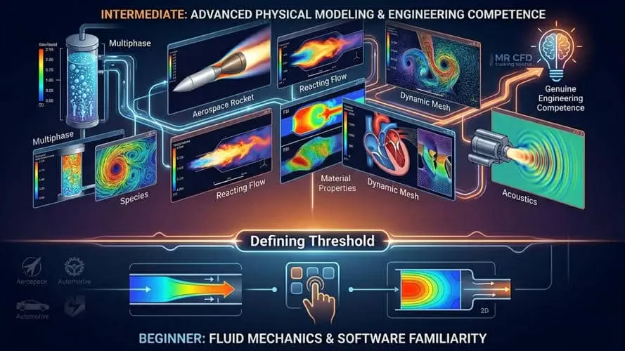
Through MR CFD’s structured CFD training course, learners engage with the full depth of intermediate CFD simulation physics across aerospace, HVAC, marine, renewable energy, turbomachinery, biomedical, chemical, and urban applications, covering multiphase and free-surface flow, compressible and reacting flow, dynamic mesh, MRF/SRF rotating systems, DPM, species transport, radiation, porous media, PCM phase change, acoustics, and an introduction to fluid-structure interaction (FSI).
Why Intermediate CFD Course (Physics Mastery) Is the Career-Defining Inflection Point
The gap between a beginner who follows guided simulations and an engineer who independently configures, troubleshoot, and validates complex models is precisely where most CFD careers stall. Industry hiring managers consistently report that competency limited to laminar flow and single-phase heat transfer is insufficient for roles in product development, thermal management, and process engineering. Employers demand engineers who understand multiphase flow dynamics, can configure turbulence-radiation interaction, and know when to apply a Moving Reference Frame (MRF) versus a sliding mesh approach.
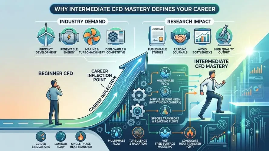
From a research standpoint, the majority of publishable CFD studies in leading journals involve at least one intermediate-level physics module , whether VOF free-surface modeling, species transport in reacting flows, or conjugate heat transfer (CHT) coupling. Researchers who cannot configure these models independently create bottlenecks in publication timelines and research output quality.
Industrially, sectors including renewable energy, turbomachinery, marine hydrodynamics, and HVAC system design are rapidly expanding CFD requirements as computational costs fall and regulatory validation demands rise. Engineers with verified intermediate ANSYS Fluent training across multiple physics modules are measurably more deployable and more competitive in both hiring and promotion cycles.
Core Technical Competencies You Will Build in This Intermediate CFD Training Course
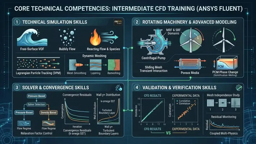
Technical Simulation Skills:
Configuring multiphase flow models, VOF, Mixture, and Eulerian frameworks, for free-surface, bubbly, and stratified flow
Setting up compressible flow simulations with density-based solvers, shock-capturing schemes, and inlet turbulence intensity boundary specifications
Implementing reacting flow and species transport models with eddy-dissipation combustion chemistry and species mass fraction boundary conditions
Applying the Discrete Phase Model (DPM) with Lagrangian particle tracking, turbulent dispersion, and heat-mass transfer coupling
Configuring dynamic mesh simulations using smoothing, layering, and remeshing with mesh motion UDF implementation
Rotating Machinery & Advanced Modeling Skills:
Setting up MRF and SRF rotating domain simulations for fans, pumps, compressors, and wind turbines
Applying sliding mesh interfaces for transient rotor-stator interaction in turbomachinery CFD simulation
Modeling PCM phase change with non-equilibrium latent heat and solidification-melting physics
Configuring porous media with Darcy-Forchheimer resistance coefficients for packed beds and heat exchangers
Solver & Convergence Skills:
Selecting between pressure-based coupled solver and density-based solver based on flow regime and Mach number
Managing wall y-plus near-wall treatment for k-omega SST and high-Reynolds turbulence models
Diagnosing multiphase and dynamic mesh convergence instabilities through relaxation factor and time-step control
Validation & Verification Skills:
Benchmarking results against experimental correlations and published engineering data
Interpreting convergence residual monitoring across coupled multi-physics simulations
Applying mesh independence studies with Reynolds-averaged Navier-Stokes (RANS) turbulence closure
Comprehensive Intermediate CFD Course Modules & Advanced Simulation Projects
Aerospace Aerodynamics Intermediate CFD Course: Intermediate Compressible Flow Analysis
This module advances into compressible flow CFD simulation at transonic and supersonic conditions. Students configure density-based solvers, apply Roe flux-difference splitting, and analyze shock wave formation, boundary layer separation, and pressure coefficient distributions , skills directly applicable to aircraft wing design, missile aerodynamics, and high-speed vehicle development.
HVAC & Building Thermal Systems CFD Course: Conjugate Heat Transfer and Radiation Coupling
Students introduce CHT coupling between building envelope components and internal airflow, combined with radiation heat transfer from solar gain and surface emissivity. Buoyancy-driven natural convection with Boussinesq approximation is configured alongside occupancy-based heat source distributions, with thermal comfort evaluation using PMV and PPD indices , directly applicable to building energy certification and smart HVAC design.
Marine Hydrodynamics Intermediate CFD Course: VOF Free-Surface Flow Simulation
This module delivers VOF free-surface modeling for ship hull resistance, wave interaction, and offshore platform hydrodynamics. Students configure two-phase VOF with geometric interface reconstruction, apply open channel flow boundary conditions, and extract drag coefficient and wave resistance outputs , skills that transfer directly to naval architecture and coastal engineering workflows.
Renewable Energy Systems: Rotating Turbine and Solar Thermal CFD
Intermediate renewable energy simulation demands MRF rotating domain configuration for wind and tidal turbine performance, combined with radiation-coupled thermal simulation for solar collectors and PV thermal management. Students configure sliding mesh interfaces for transient blade passage analysis and evaluate power coefficient curves and thermal efficiency metrics applicable to wind farm and solar thermal plant design.
Turbomachinery: MRF, SRF, and Sliding Mesh Rotating Systems
The most technically demanding module in the intermediate curriculum. Students progress from SRF isolated rotor analysis through MRF multi-zone stage performance prediction to transient sliding mesh rotor-stator interaction simulations. Pump characteristic curves, compressor surge margins, and fan noise outputs are extracted and validated against manufacturer data , building skills directly applicable to turbomachinery design and certification.
Biomedical Engineering: Pulsatile Flow and Particle Transport
This module introduces pulsatile non-Newtonian flow in cardiovascular geometries and DPM Lagrangian particle tracking for drug delivery and aerosol deposition in respiratory airways. Students configure cardiac waveform inlet profiles, apply Carreau and Power-Law viscosity models for blood rheology, and track particle deposition efficiency , competencies demanded in medical device regulatory submissions and pharmaceutical inhaler development.
Chemical Engineering: Species Transport and Reacting Flow Systems
Students advance into species transport and reacting flow CFD for chemical process equipment. Multi-species inlet boundary conditions with species mass fraction specifications are configured alongside eddy-dissipation combustion models, with analysis of mixing efficiency, reaction zone temperature profiles, and pollutant concentration fields, spanning industrial burner design, reactor optimization, and emissions compliance.
Urban Airflow & Environmental CFD: Atmospheric Boundary Layer Simulation
This module introduces atmospheric boundary layer (ABL) inlet profiles, urban canopy roughness modeling, and buoyancy-coupled outdoor thermal comfort analysis. Students configure logarithmic wind profiles, apply surface roughness parameters, and evaluate pedestrian-level wind velocity and thermal comfort indices applicable to urban planning consultancy and wind microclimate assessment.
Dynamic Mesh & Moving Boundary Simulations
One of the most technically challenging modules, covering valve motion, piston reciprocation, and flexible structure deformation. Students implement mesh motion UDFs in C, configure spring-based smoothing and local remeshing, and manage mesh quality throughout transient cycles, establishing the foundational competency for advanced FSI work at the expert level.
Acoustics: Flow-Induced Noise and Pressure Fluctuation Analysis
Acoustics CFD simulation in ANSYS Fluent applies the Ffowcs Williams-Hawkings (FW-H) acoustic analogy to predict far-field noise from turbulent flow over surfaces and rotating blades. Students configure acoustic receivers, extract sound pressure level (SPL) spectra, and identify tonal and broadband noise sources, directly applicable to HVAC noise compliance, wind turbine certification, and automotive aeroacoustics.
Phase Change (PCM) and Solidification-Melting Simulations
PCM CFD simulation requires accurate modeling of non-equilibrium latent heat during solid-liquid transitions. Students configure Fluent’s solidification-melting model with mushy zone parameters, apply CHT coupling between PCM and container walls, and evaluate charge-discharge cycle performance, applicable to thermal energy storage, electronics cooling, and concentrated solar power systems.
Introduction to Fluid-Structure Interaction (FSI) in ANSYS
This module bridges fluid dynamics and structural mechanics by coupling ANSYS Fluent with ANSYS Mechanical for one-way and two-way structural coupling. Students configure fluid pressure load transfer, apply mesh motion driven by structural deformation, and analyze deflection and stress in flow-loaded components, establishing the framework for the expert-level FSI curriculum.
ANSYS CFX and Discovery: Extending Beyond Fluent
The course concludes with an extension module introducing ANSYS CFX and ANSYS Discovery, providing comparative solver awareness. Students explore CFX’s coupled solver architecture for rotating machinery and multiphase applications, and use Discovery’s real-time simulation capabilities for rapid design exploration within a unified ANSYS Workbench workflow.
Professional Engineering Skills Developed Through Intermediate CFD Simulation Training
Skill Category | Competencies Acquired |
Multiphase Flow Modeling | VOF free-surface, Eulerian multiphase, Mixture model, cavitation, DPM particle tracking |
Rotating Machinery CFD | MRF, SRF, sliding mesh, fan/pump/compressor performance curve extraction |
Reacting & Compressible Flow | Species transport, eddy-dissipation combustion, density-based solver, shock capturing |
Thermal & Radiation Coupling | CHT conjugate transfer, radiation-convection coupling, PCM solidification-melting |
Dynamic & Moving Mesh | Spring smoothing, layering, remeshing, UDF mesh motion, FSI coupling introduction |
Acoustics & Vibration | FW-H acoustic analogy, SPL spectrum extraction, flow-induced noise identification |
Solver & Convergence Mastery | Pressure-based coupled solver, y-plus management, residual diagnostics, time-step control |
Post-Processing & Reporting | Force coefficient extraction, contour and vector visualization, XY plot analysis, animation |
Real-World Industrial Applications of Intermediate CFD Simulation Competency
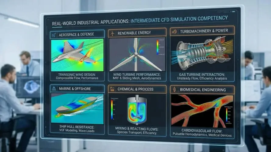
Aerospace & Defense: Transonic aerodynamic analysis, compressible flow over control surfaces, acoustic noise prediction for propulsion systems
Renewable Energy: Wind turbine rotor performance using MRF and sliding mesh, solar collector thermal optimization, tidal turbine hydrodynamic analysis
Turbomachinery & Power Generation: Pump and compressor characteristic curve prediction, fan aeroacoustics, gas turbine stage interaction analysis
Marine & Offshore Engineering: Ship hull resistance via VOF free-surface modeling, offshore platform wave loading, propeller performance simulation
HVAC & Building Systems: Solar gain-coupled thermal comfort analysis, natural convection HVAC optimization, radiant heating simulation
Chemical & Process Engineering: Reacting flow reactor design, species mixing efficiency analysis, combustion pollutant prediction
Biomedical Engineering: Cardiovascular pulsatile flow analysis, respiratory aerosol deposition, medical device flow characterization
Urban & Environmental Engineering: Atmospheric boundary layer wind simulation, pedestrian comfort assessment, urban heat island mitigation
Who Should Enroll in This Intermediate ANSYS Fluent Comprehensive Training
Engineering Students Who Have Completed a Beginner CFD Course: Students who have finished the Beginner CFD Course (First Level of ANSYS Fluent Course) course and are ready to advance beyond guided projects into independent, analytically demanding intermediate CFD simulation work across multiple physics domains.
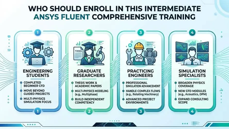
Graduate Researchers & PhD Candidates: Researchers who need to configure multi-physics CFD models for thesis work, including multiphase flow, reacting flow, or FSI simulations , and require structured training to build the independent modeling competency that academic supervisors and journal reviewers expect.
Practicing Engineers Seeking Simulation Advancement: Mechanical, chemical, aerospace, and energy engineers with basic ANSYS Fluent exposure who need structured training to confidently handle rotating machinery, compressible flow, dynamic mesh, and species transport simulations in professional project environments.
Simulation Specialists Broadening Physics Coverage: CFD analysts proficient in one or two physics domains who need systematic exposure to the full range of intermediate CFD simulation modules from acoustics and PCM phase change to DPM and atmospheric boundary layer modeling to expand project scope and consulting capability.
Why MR CFD Delivers Unmatched Authority for Intermediate Simulation Mastery
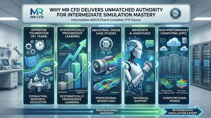
Over 15 years of continuous CFD consulting, research, and structured engineering education underpin every aspect of this course. Key differentiators include:
Structured Progression Architecture: Every project is calibrated to be one measurable step harder than its beginner equivalent , systematically more demanding in model configuration, boundary condition judgment, and result interpretation.
Production-Grade Simulation Standards: All case studies reflect the same quality standards applied in MR CFD’s industrial consulting engagements, ensuring learners develop workflows that transfer directly to professional environments.
AI-Assisted Technical Support: Immediate, technically precise answers to simulation questions throughout the course via MR CFD’s AI-assisted support system.
HPC Computing Access: For computationally intensive cases, transient sliding mesh, VOF free-surface, and reacting flow simulations, learners leverage ANSYS HPC without local hardware constraints.
15 Years of Consulting Expertise: Practical engineering judgment and troubleshooting intuition embedded from MR CFD’s portfolio of industrial and research CFD projects.
For project-specific simulation support beyond the training curriculum, MR CFD’s CFD consulting services provide expert-led engagement across all intermediate and advanced physics domains.
Learning Progression Path: From Intermediate CFD to Expert-Level Simulation
Stage | Course | Physics Scope |
Beginner | 47 introductory projects across 17 engineering fields and basic Fluent modules | |
Intermediate | Intermediate ANSYS Fluent Complete CFD Course | Multiphase, compressible, reacting, dynamic mesh, DPM, acoustics, PCM, FSI intro |
Expert | Become an Expert ANSYS Fluent User | Full multi-physics coupling, advanced turbulence models, optimization, research-grade validation |
Upon completing this course, learners are fully prepared to pursue expert-level specialization in thermal management, multiphase flow, aerodynamics, combustion, battery thermal simulation, fuel cell CFD, FSI, and design optimization. The CFD Internship Program provides a structured pathway for intermediate graduates to apply simulation competencies in real consulting project environments, building a verifiable professional portfolio.
Advance Your CFD Engineering Career, Enroll in the Intermediate Course Today
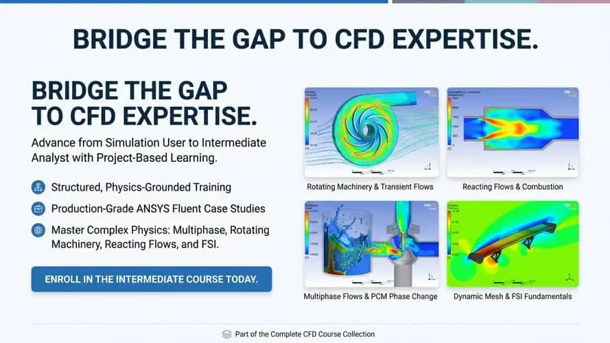
The difference between an engineer who runs simulations and one who understands them is built at the intermediate level. The Intermediate ANSYS Fluent Complete CFD Course delivers the structured, physics-grounded, project-based training that makes that difference concrete and measurable , spanning multiphase flow, rotating machinery, compressible and reacting flows, dynamic mesh, acoustics, PCM phase change, and FSI fundamentals through production-grade ANSYS Fluent case studies.
Continue your structured simulation learning path through CFD training Course collection and advance from competent beginner to confident intermediate analyst today.
This is the direct sequel to Start Learning CFD Simulation by ANSYS Fluent, and it assumes you already know the basic Fluent workflow (build geometry, mesh, set up the solver, read results). If you can run a simple case on your own, you can start here. If you are brand new to CFD, take the beginner course first, then level up with this one.
It follows the same map of engineering fields, flow models, and Fluent modules, but adds a second, more demanding project to every topic. Where the first course showed you the basic version of each idea, this one pushes into harder physics, larger meshes, transient solvers, and multi-physics coupling. Think of it as the same tour, walked at a deeper level.
Quite a few. You move into the adjoint solver and RBF mesh morphing for shape optimization, radiation modeling (including solar load on a building), porous media, phase change material (solidification and melting), single and moving reference frames on a centrifugal compressor, vortex shedding (the Von Kármán effect), heat pipe evaporation and condensation, a transient combustion chamber, and an introduction to ANSYS Discovery. These are the tools that separate a beginner from a working CFD engineer.
It is for engineers and students who have the fundamentals down and now want to handle realistic, industry-style problems. If you have finished an introductory course or already run basic simulations at work or university, this is the natural next step toward real multi-physics analysis.
You will need ANSYS installed on your side, including ANSYS Fluent plus the geometry and meshing tools used across the lessons (Design Modeler, SpaceClaim, ANSYS Meshing, and Fluent Meshing). One module also uses ANSYS Discovery. The course teaches the workflow inside ANSYS, so an active ANSYS license (student or commercial) is what you bring.
Yes, they are heavier. Several cases use large meshes and transient solvers, which take real compute time and memory. A modern workstation handles most of them, but the largest transient and multi-physics runs are far more comfortable on dedicated hardware, which is where the HPC option below comes in.
No. Each project stands on its own, so you can jump to the field, model, or module you care about. Because the difficulty steps up, just make sure you are comfortable with the basic Fluent workflow before diving into the advanced modules like FSI, combustion, or the adjoint solver.
The compressor and fan lessons map to turbomachinery and HVAC, the radiation and PCM lessons to building energy and thermal storage, the porous media and heat pipe lessons to electronics cooling and process equipment, the FSI and dynamic mesh lessons to moving bodies like valves and projectiles, and the urban pollution and species transport lessons to environmental engineering. Each project points out where its workflow reappears in industry.