

MHD Effect on Fluid Flow CFD Simulation, ANSYS Fluent Training
Price: $36
The present problem simulates a fluid flow with electrical conductivity properties in a simple square chamber.
MHD Effect on Fluid Flow CFD Simulation, ANSYS Fluent Training
Price: $36
The present problem simulates a fluid flow with electrical conductivity properties in a simple square chamber.

MHD Project Description
The present problem simulates a fluid flow with electrical conductivity properties in a simple square chamber by ANSYS Fluent software. The MHD model was used to model this work. Magnetohydrodynamics (MHD) is a science that studies the magnetic properties of electrically conductive fluids. In fact, the MHD deals with the interaction between magnetic particles within a fluid stream and the magnetic field. In this case, the fluid flow field and the magnetic field are combined, which is influenced by the induction of electric current due to the movement of the conductive material in a magnetic field, as well as the Lorentz force due to the interaction of the magnetic field and the electric current.
The MHD model is defined in the present simulation by magnetic induction method. This MHD definition method includes two user-defined scalar magnetic flux field functions in the x and y directions; The electrical potential method, on the other hand, involves a voltage scalar function. For the four boundaries of the computational area of the problem, the boundary condition of the insulating wall type is defined; This means that no electric current is transmitted at these boundaries.
Project Description
This is from the conducting wall boundary condition to define fully conductive boundaries, from the coupled wall boundary condition to define the common boundaries between solid and solid or liquid and solid, and from the wall boundary condition. A thin wall is used to define the boundary condition of limited electrical conductivity. In the present magnetic field simulation, the energy equations, the Lorentz force equations, and the MHD equations are activated, and accordingly, to define the magnetic field in the model, a source term for energy, momentum, and magnetic fluxes are applied.
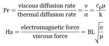
The present problem first examines the dimensionless Prandtl number without applying the MHD model; That is, it examines the ratio of diffusion of motion size to thermal penetration in the model. It then examines the Hartmann number at a constant value of the Prandtl number, followed by the magnitude of the magnetic flux in the presence of MHD; It examines the ratio of electromagnetic force to viscosity force in the model. Finally, at a constant value of the Hartmann number, it examines the changes in the angle of application of the magnetic flux to the fluid flow.
Project Description
To define the desired fluid, from density equal to 998.2 kg.m-3, thermal conductivity equal to 0.6 Wm-1.K-1, dynamic viscosity equal to 0.001003 kg.m-1.s-1, thermal expansion coefficient of 0.000214 K-1, and an electrical conductivity of 1000000 siemense.m-1 (s3.A2.kg-1.m-2) were used. Now, according to the formula for the Prandtl number, the amount of specific heat capacity causes the Prandtl number to change. The value of Prandtl in different models includes 0.01, 0.02, 0.03 and 0.004. Also, according to the Hartmann number formula, the amount of magnetic flux applied causes the Hartmann number to change.
The value of the Hartmann number in different models includes 0.003284, 0.006568, 0.013135, and 0.032838. This value of Hartmann changes with the magnitude of the magnetic flux applied to the model, but this amount of magnetic flux is applied at a certain angle (vertically and only in the direction of the y-axis). In the final part of the work, assuming the amount of magnetic flux is constant, different directions are considered for applying the magnetic field, including an angle of zero degrees (horizontally and only in the direction of the x-axis), an angle of 45 degrees with The x-axis is at an angle of 60 degrees to the x-axis and the 90-degree angle (vertically to the y-axis only).
(MHD)
Geometry & Mesh
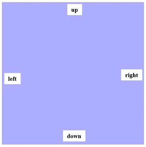
The present 2-D model is drawn using Design Modeler software. The present model consists of a square computing space with a side of one meter, which consists of four walls including up, down, left and right. The following figure shows a view of the geometry.
(MHD)
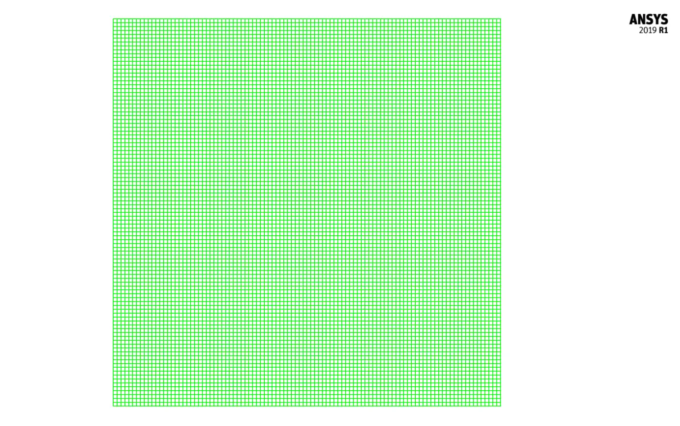
The meshing of the model has been done using ANSYS Meshing software and the mesh type is structured. The element number is 10000 . The following figure shows the mesh.
MHD CFD Simulation Setting
To simulate the present model, we consider several assumptions:
- We perform a pressure-based solver.
- The simulation is steady.
- The gravity effect on the fluid is not considered.
We present a summary of the defining steps of the problem and its solution in the following table:
| (MHD) | Models | |
| Viscous model | Laminar | |
| Energy | on | |
| (MHD) | Boundary conditions | |
| down wall | Wall | |
| wall motion | stationary wall | |
| temperature | 587 K | |
| left & right | (MHD) | Pressure outlet |
| wall motion | stationary wall | |
| heat flux | 0 W.m-2 | |
| up wall | Wall | |
| wall motion | stationary wall | |
| temperature | 300 K | |
| (MHD) | Solution Methods | |
| Pressure-velocity coupling | SIMPLE | |
| Spatial discretization | pressure | second order |
| momentum | second order upwind | |
| energy | second order upwind | |
| (MHD) | Initialization | |
| Initialization method | Standard | |
| gauge pressure | 0 pascal | |
| temperature | 443.5 K | |
| x-velocity, y-velocity | 0 m.s-1 |
MHD Results
At the end of the solution process, we obtain two-dimensional counters of pressure, velocity, and temperature, as well as two-dimensional pathlines in three different simulation steps. The first step is without applying the MHD model and we compare the Prandtl number and consequently the amount of dynamic viscosity in four different values. The second step is by defining the MHD model and assuming a constant Prandtl number, we compare the value of the Hartmann number and consequently the magnitude of the magnetic flux in four different values but in a fixed direction.
In the third step, by defining the MHD model, assuming the Prandtl number as well as the constant Hartmann number, we compare the direction of applying the magnetic flux in four different angles but with a constant value.