NACA0012 Airfoil Optimization With RBF Morph, CFD Simulation Ansys Fluent Training
Price: $31.50
In this project, a NACA0012 Airfoil with the RBF (Mesh Morphing) Method has been simulated, and the results of this simulation have been investigated.
NACA0012 Airfoil Optimization With RBF Morph, CFD Simulation Ansys Fluent Training
Price: $31.50
In this project, a NACA0012 Airfoil with the RBF (Mesh Morphing) Method has been simulated, and the results of this simulation have been investigated.
NACA0012 Airfoil Optimization Project Description
In this project, the flow inside a NACA0012 airfoil is first has been simulated by Ansys Fluent software. The angle of attack is 1.53 degrees, and the simulation has been done by the density-based solver due to the compressibility with a Mach number equal to 0.7. Then the geometry is optimized to improve lift-to-drag (L/D) as aerodynamic efficiency. All the optimization has been done by Ansys Fluent software in the Ansys Workbench environment.
The optimization step is performed in three stages. In the first stage, only the displacement of points in the vertical direction was considered, and the best answers were obtained for the maximum lift-to-drag ratio and maximum lift coefficient. Then in the next step, each of these two optimal solutions was considered for horizontal displacement, and the lift-to-drag ratio was obtained in two new modes.
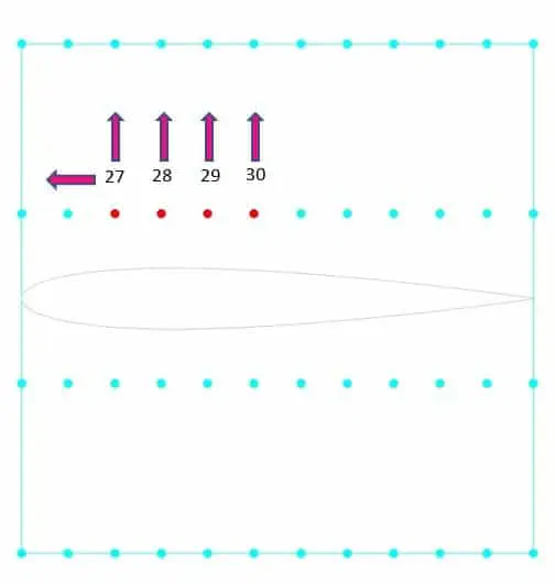
For this purpose, an area is defined around the airfoil, the center of which is (0,-0.5), with the regular control point distribution. The update from the zone is set for the airfoil walls, and this wall's constraint type is set to unconstrained type. The length and the height of this rectangle are 1 meter. The number of nodes in the X-direction is 12, and the number of nodes in the Y-direction is 4. In fact, the input parameter for this optimization is the vertical and horizontal displacement of these points.
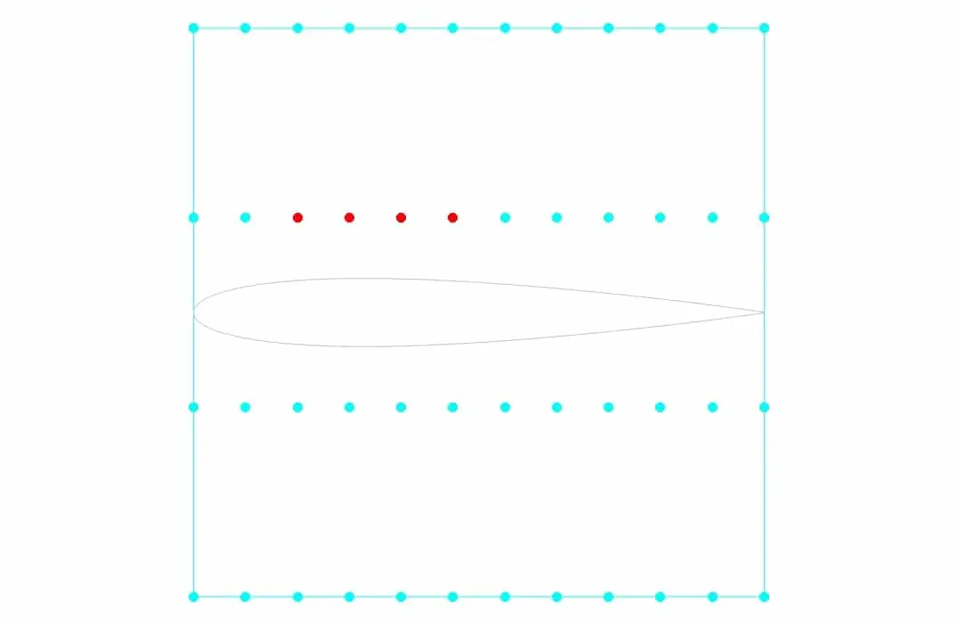
The constraint for another boundary (Farfield) is set to fix. To begin the optimization process, you have to define the motion for each of these points. In this project, for points numbers, 28,29, and 30, the displacement to the +y is considered, and for point 27, the displacement to both -x and +y directions is considered. In the first stage, no horizontal displacement is considered, and the optimal result is obtained only based on vertical displacement. Then, in the next step, based on the best answer of the lift and drag ratio, the amount of vertical displacement is selected. Horizontal displacement is then applied and optimized for vertical displacement to obtain the best lift-to-drag ratio. This optimization has been done once for the best lift coefficient. Finally, the results are compared.
Geometry & Mesh
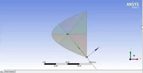
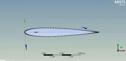
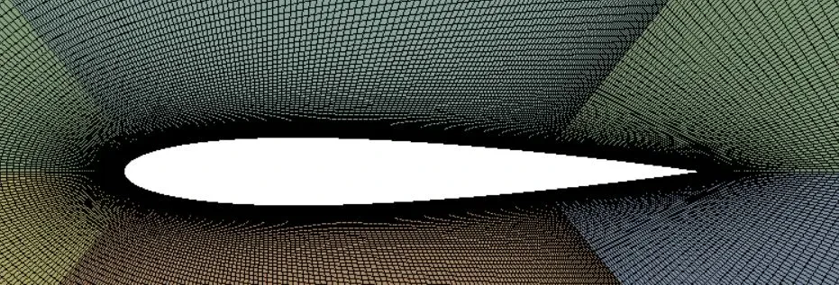
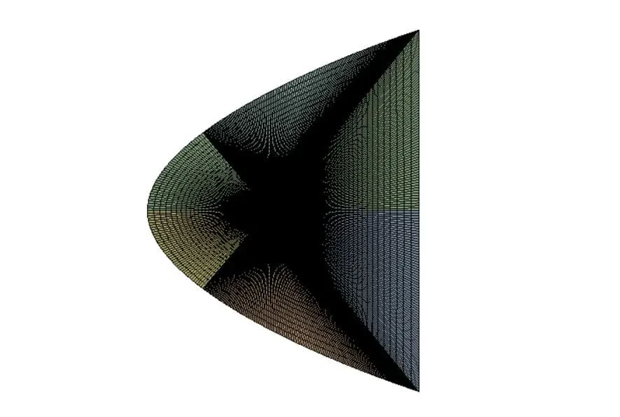
The geometry is designed by the Design Modeler Software, and the meshing of this model has been generated by Ansys Meshing software. The grid type is structured and the total cell number is 73320.
NACA0012 Airfoil CFD Simulation
To simulate the present model, several assumptions are considered, which are:
- The solver is density-based due to compressibility.
- Simulation has been done as steady-state.
- The gravity effect has been neglected.
The following is a summary of the steps for defining the problem and its solution:
| Models | ||
| Viscous | Spalart Allmaras | |
| Spalart Allmaras Production | Strain/Vorticity-based | |
| Boundary conditions | ||
| Farfield | Mach Number | |
| Pressure Fairfield | 0.7 X-component of flow direction: 0.9996435 Y-component of flow direction: 0.02670036 | |
| Airfoil Up & Airfoil Bottom | Wall | |
| Wall motion | Stationary Wall | |
| Shear Condition | No-slip condition | |
| Methods | ||
| Formulation Flux type | Implicit Roe-FDS | |
| Flow & Modified turbulent viscosity | Second-order upwind | |
| gradient | Green Gauss Node-based | |
| Initialization | ||
| Initialization methods | Standard | |
| Compute from | Far-field | |
| Material | ||
| Material properties | ||
| density | Ideal gas | |
| viscosity | Sutherland | |
| Cp | 1006.43 | |
NACA0012 Airfoil Optimization Results
First Step Optimization
After optimization, we were able to obtain the optimum points for the maximum lift-to-drag ratio. The table and plots below show the first step of optimization.
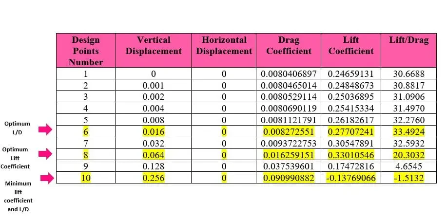
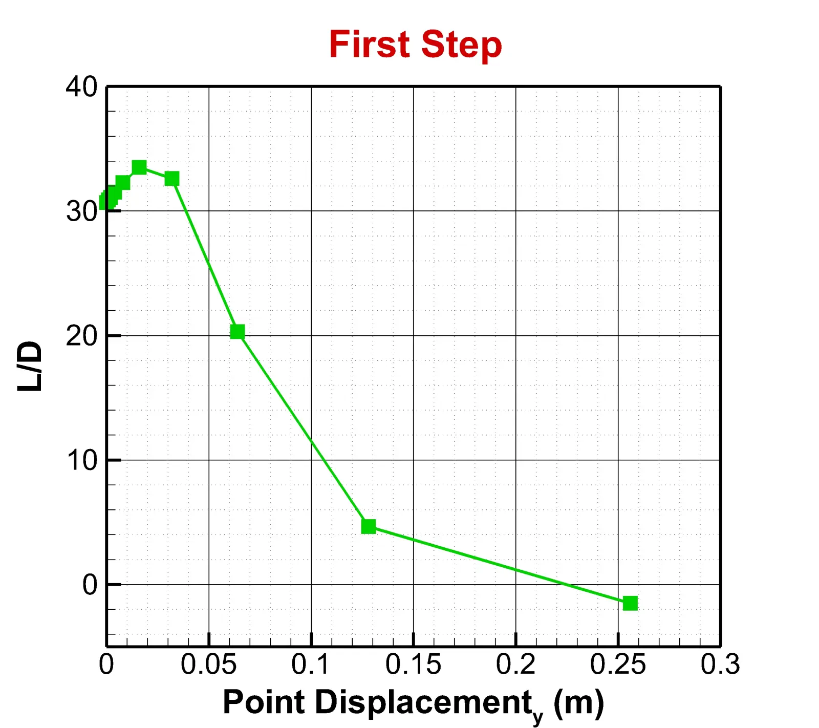
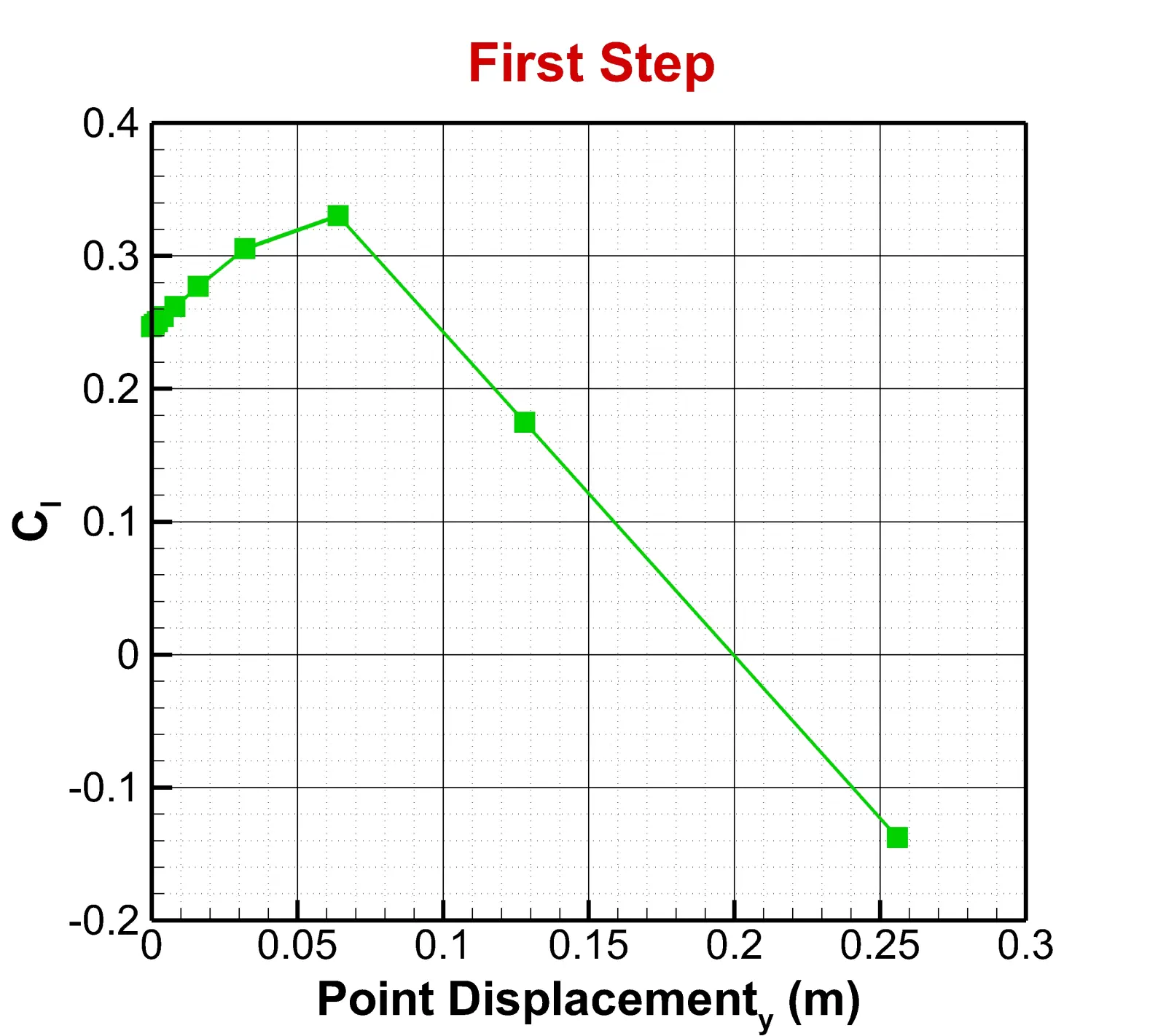
As can be seen from the table above, the highest lift-to-drag ratio has occurred in 0.016 m vertical displacement, and the highest lift ratio has occurred in 0.064 m vertical displacement. Also, at a vertical displacement of 0.256 m, the amount of lift force is negative, and the lowest value compared to other displacements is obtained for both the lift-to-drag ratio and the lift coefficient.
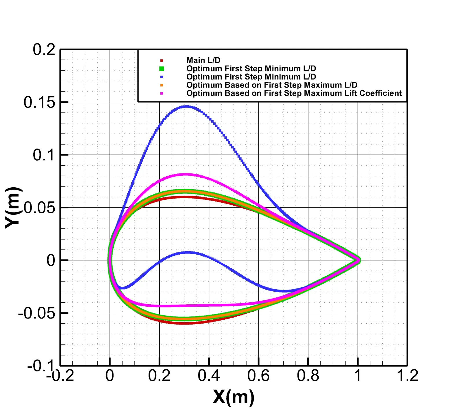
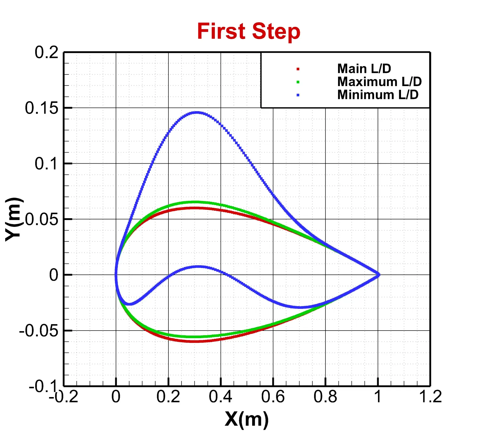
The image below shows a vertical coordinate diagram of the airfoils in the case related to the maximum L/D and case related to the minimum L/d and optimized state relative to their horizontal coordinates; in fact, this is a schematic diagram that shows how the geometry of the airfoil has changed.
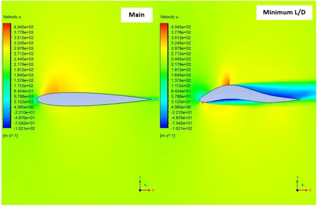
Below the velocity contour in the X direction has been drawn for the maximum and minimum lift-to-drag modes. As it is known, in the first case, as the upper surface of the airfoil is pulled upwards, the force difference between the upper and lower levels of the airfoil increases, and as a result, the lift force increases. On the other hand, the velocity on the upper surface of the airfoil has increased, which in turn has delayed the separation of the flow.
In the second case, the shock is observed on the upper surface of the airfoil, which is almost a normal shock. As it is known, after this shock, the flow velocity has suddenly decreased, which has intensified the separation in this area. On the other hand, due to the concavity created in the lower surface of the airfoil, the difference between the forces of the upper and lower levels of the airfoil has caused a negative lift.
Second Step Optimization
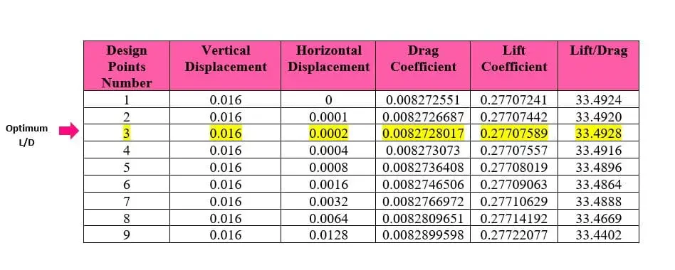
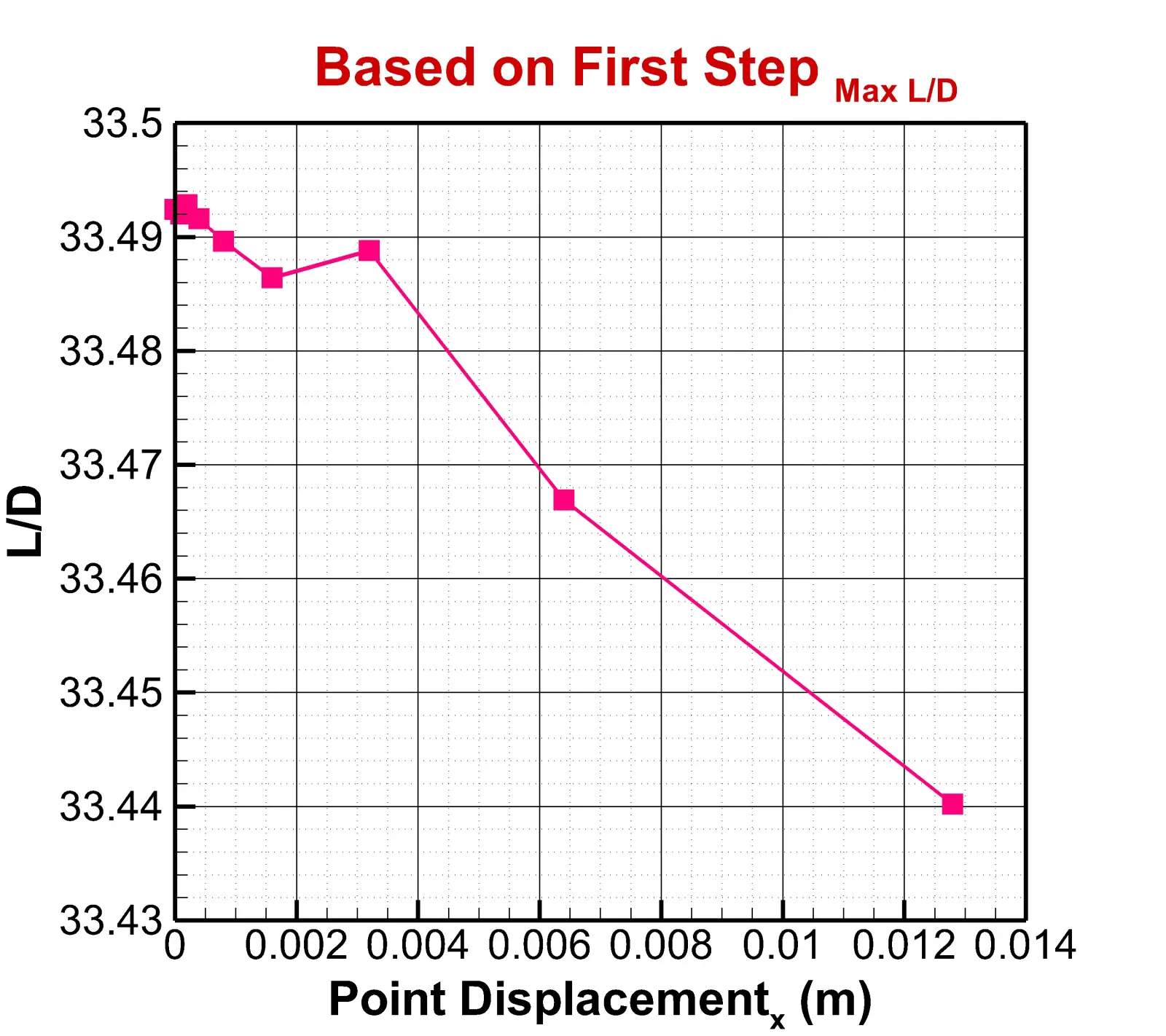
The table and plot below show the second stage of optimization. In the situation where the best vertical displacement for the highest lift-to-drag ratio is selected from the previous stage and in this stage, horizontal displacement is considered.
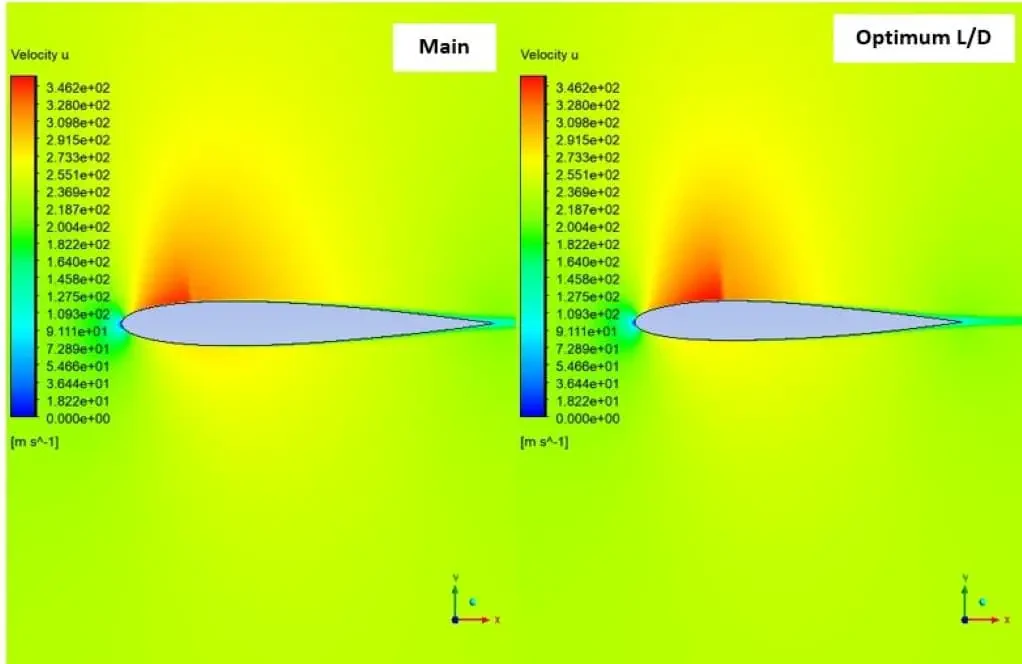
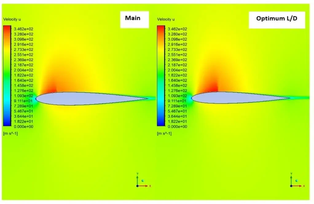
The following contour shows that, as in the first step, the separation of the flow is delayed, and the velocity on the upper surface is increased. Also, as it is clear, the changes in this mode are very small compared to the optimal mode of the first stage.
Third Step Optimization
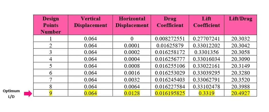
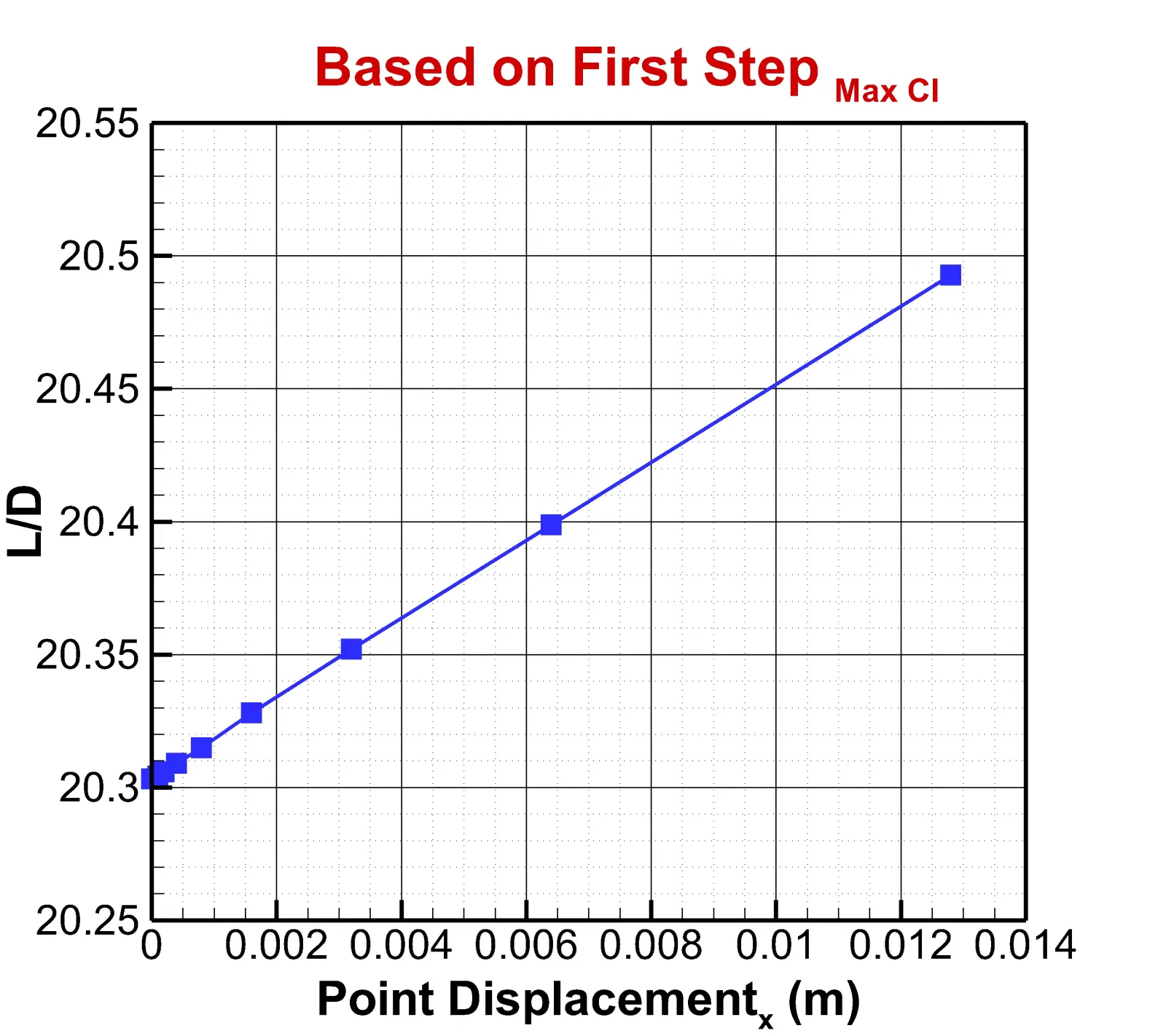
In the last step, the optimization is performed based on the vertical displacement of the maximum amount of lift in the first step. The table and diagram below show information about this optimization.
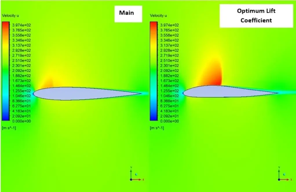
The velocity contour for step 3 is drawn below. As you can see, like the previous steps, the shock is bigger. The reason for this is the change in the airfoil bend in the specified areas. Also, due to the change in the symmetry of the airfoil shape, the lift force has increased.
Finally, the vertical coordinate diagram of the airfoils in the initial and optimized state relative to their horizontal coordinates is drawn below.