Pollutant Distribution from Car Exhaust in Static and Traffic (Low-Speed) Modes
Price: $140
In this research, using species transport module, the gases from combustion in the car engine and their interaction with the open air in the urban environment were investigated statically and in traffic mode.
Pollutant Introduction
The use of fossil fuels was always associated with various pollutant. Lack of complete combustion and production of NOx, Sox, and unburned hydrocarbons quickly causes more air pollution. Meanwhile, improving fuel production standards are reducing these pollutants day by day. For example, the standard Euro4 is much cleaner than Euro2 fuel. Now, considering that during city traffic, the speed of cars was lower and their distance was closer to each other, the amount of pollution while standing and moving at low speed can be compared. Therefore, simultaneous investigation of pollutants and environmental conditions of cars should be considered.
Problem Description
In this research, using Species Transport module, the gases from combustion in the car engine and their interaction with the open air in the urban environment were investigated statically and in traffic mode by ANSYS Fluent software. For this purpose, the exhaust gas velocity was equal to 1 m / s, and the temperature was 400 K for the static state. In the second case, with the same speed and temperature of the exhaust gas, an external flow with a 3 m / s enters due to the car's movement in traffic mode. Finally, by comparing the pollutant gases for static and traffic mode with low speeds, the distribution of exhaust pollution was studied.
Geometry & Mesh
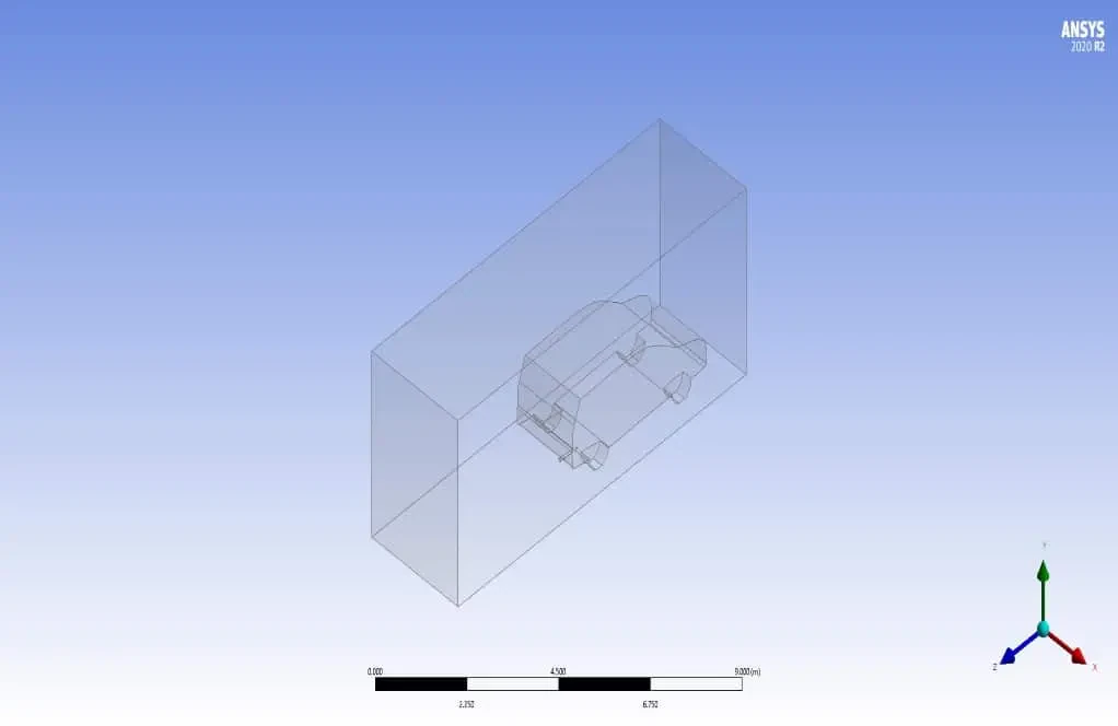
The geometry was designed using the Design Modeler module (figure below), and its geometric specifications include a car and fluid domain around it. For more accurate modeling of gas distribution, the rear side of the car was more extruded. The dimensions of the fluid domain around the car were 4*6*10 m.
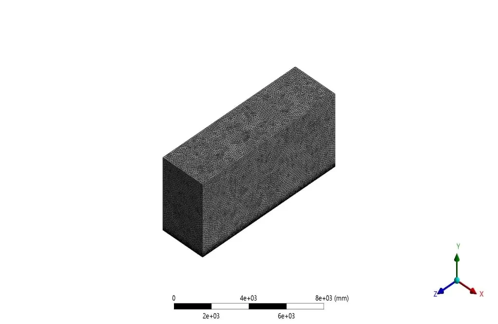
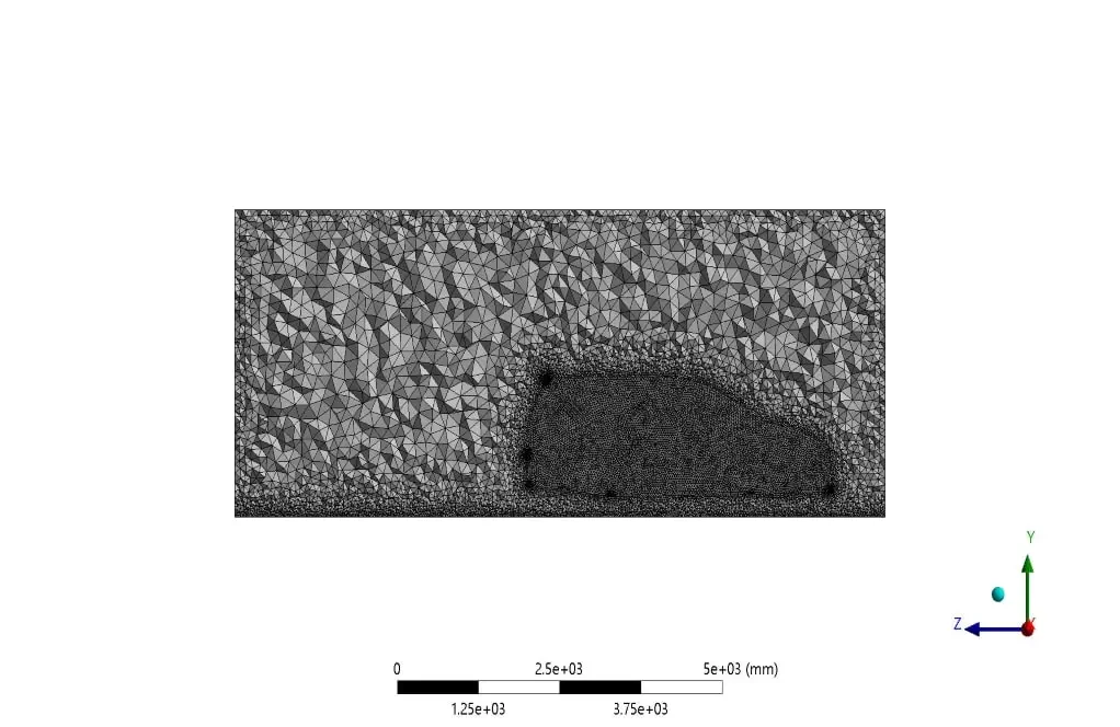
For grid generation, unstructured mesh with 3122361 elements in the ANSYS Meshing module was utilized. Curvature and proximity method was used to focus on grid sensitive areas of the solution domain. The following figure shows the mesh generation for this problem.
Solver Setting
Fluent software was used to solve the governing equations numerically. The problem is analyzed steady, using the pressure-based method, and considering the gravitational effects. Also, for solving the above problem, a combination of RANS and species transport equations was used to study the simultaneous effect of combustion gases and their combination with air in the computational domain.
Pollutant Material Properties
Pollutant gases enter the fluid domain as a mixture material containing NO2, NO, SO2, CO, CO2, Soot, and H2O with mass fraction percentages proportional to the type of pollutant input from the exhaust section. Air is also used as a solution domain fluid with fixed properties in the software.
Boundary conditions and Solution methods
Also, The table below shows the characteristics and values of boundary conditions, along with the models and hypotheses.
| Material Properties | |||
| Amount | Fluid properties (mixture) | ||
| Incompressible ideal gas | Density | ||
| Mixing law | Specific heat | ||
| 0.0454 | Thermal conductivity (w/m.K) | ||
| 0.0000172 | Viscosity (kg/m.s) | ||
| Mass fraction input | |||
| Species mass fraction | Material name | ||
| 0.2 | CO2 | ||
| 0.04 | CO | ||
| 0.01 | SO2 | ||
| 0.00001 | NO2 | ||
| 0.00001 | Soot | ||
| 0.08 | H2O | ||
| Boundary Condition | |||
| Type | Amount (units) | ||
| Velocity inlet (mixture gas at 400 K) | 1 m/s | ||
| Velocity inlet (air at 300 K) | 3 m/s | ||
| pressure outlet (gauge pressure) | 0 pa | ||
| car wall (no slip) | Adiabatic (heat flux=0 W/m2) | ||
| domain wall | symmetry | ||
| Cell zone condition | |||
| Fluid | Air | ||
| Turbulence models (Toyota gas exhaust) | |||
| K- | viscous model | ||
| Standard | K- model | ||
| Standard wall | Wall function | ||
| Solution methods (Toyota gas exhaust) | |||
| Simple | pressure velocity coupling | ||
| Standard | pressure | spatial discretization | |
| Second-order upwind | momentum | ||
| First-order upwind | turbulent kinetic energy | ||
| First-order upwind | turbulent dissipation rate | ||
| Second-order upwind | energy | ||
| Second-order upwind | Species transport | ||
| Initialization | |||
| standard | initialization method | ||
| 0 (Pa) | gauge pressure | ||
| 1 m/s | z-velocity (gas exhaust) | ||
| 3 m/s | z-velocity (traffic mode external flow) | ||
| 0 (m/s) | y-velocity , x-velocity | ||
Results
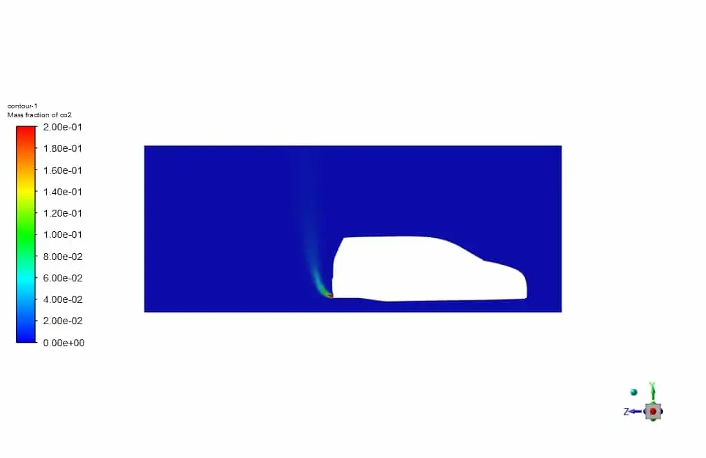
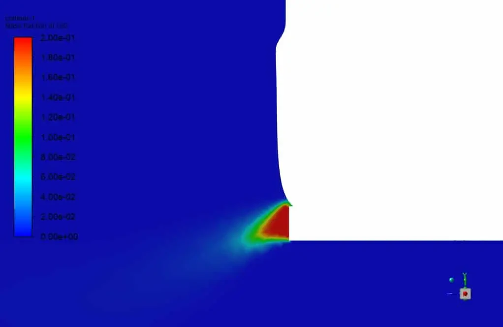
In this section, by studying the contours and streamlines obtained from the simulation, the mass distribution of the species and the effect of external flow in the solution domain were discussed. First, according to the CO2 mass fraction contours and comparing the two static and external flow (traffic mode), it is observed that the presence of external flow or so-called car movement, due to the creation of vortices in the rear, the distribution of pollutants is more horizontal and prevents them from moving rapidly into the atmosphere. The image below is for static mode.
Co2 (pollutant) Distribution for Static Mode
Co2 (pollutant) Distribution for Traffic Mode
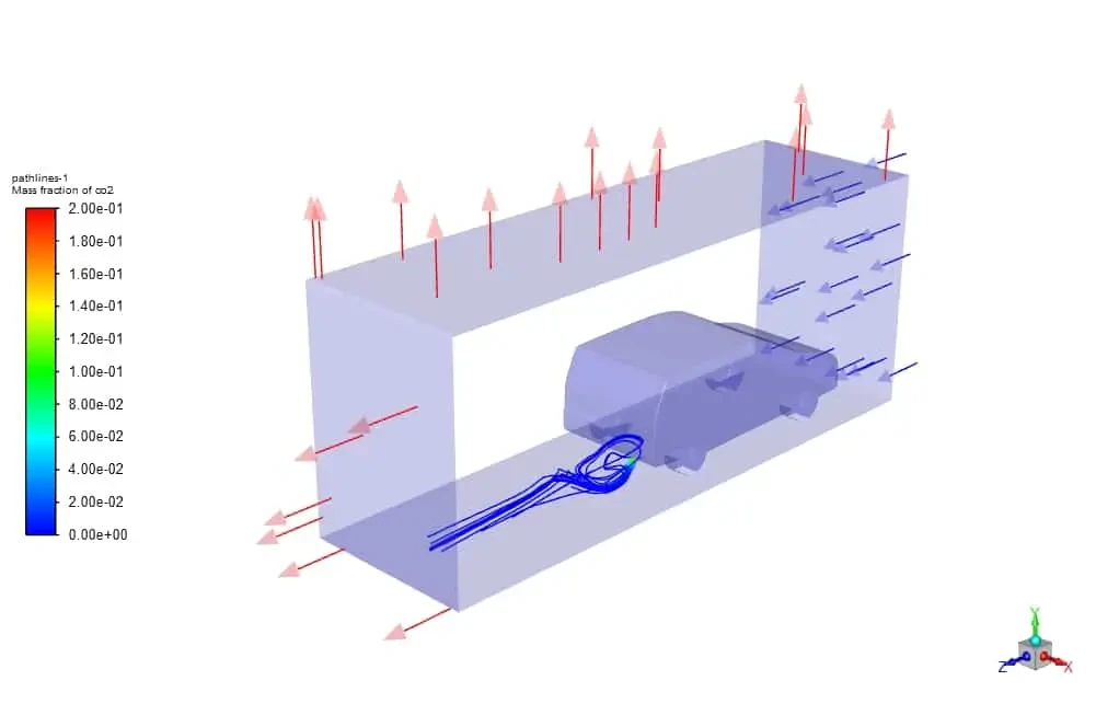
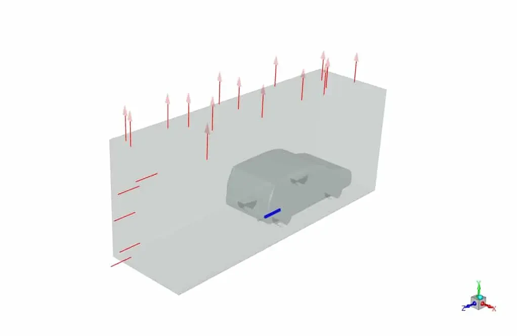
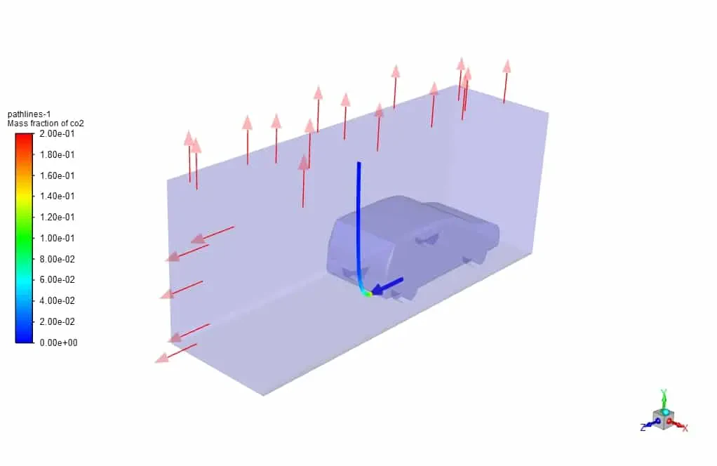
With three-dimensional comparison and using streamlines, the effect of horizontal distribution of species is better determined. In the following figures, first, there is no external flow, and then by importing the external flow, there is no opportunity for pollutant to escape to the atmosphere vertically.
Co2 Distribution for Static Mode
Co2 Distribution for Traffic Mode