

Single Reference Frame (SRF) Axial Pump CFD Simulation
Price: Free
- The problem numerically simulates the Axial Pump using ANSYS Fluent software.
- We design the 3-D model by the SpaceClaim software.
- We Mesh the model by ANSYS Meshing software, and the element number equals 36,865.
- The Single Reference Frame is defined to model rotational movement.
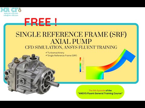

Single Reference Frame (SRF) Axial Pump CFD Simulation, ANSYS Fluent Training
Description
In this project, which has been done with CFD numerical simulation method, an axial pump is simulated. In axial pumps, the fluid flow is in the direction of the impeller shaft axis. Of course, there are different types of axial pumps. The flow direction in them can be between the radial and axial directions.
Axial pumps should be used where high fluid flow and low head are required. In this project, the inlet speed of water is 2 m/s and the outlet is atmospheric pressure. The rotational speed of the pump impeller is 200 rpm, and the Frame Motion module has been used.
The two-dimensional geometry has been produced with SpaceClaim software. The length of the commutating domain is 118 mm, and the width is 117 mm. In addition, The meshing has been done with ANSYS Meshing software, and the type of elements is unstructured. Also, the total number of elements is 36,865.
This CFD project is the 9th episode of the ANSYS Fluent General Training Course.
Methodology: Single Reference Frame (SRF) Axial Pump
The pressure-based solver is employed due to the incompressibility of the water. The gravitational acceleration is ignored. Also, the simulation is performed in steady form. It should be mentioned that the Axisymmetric Swirl option is used. The rotational motion of the flow is modeled by MRF.
Conclusion
After the simulation, we can see that due to the blade's rotational speed, the radial component of the velocity at the output increases relative to the input. Also, the dynamic pressure, which is directly related to the velocity of the fluid, increases accordingly.