

Tank Charge (2-Phases), CFD Simulation Ansys Fluent Training
Price: $16
In this project, a tank charge has been simulated and the results of this simulation have been investigated.
Tank Charge (2-Phases), CFD Simulation Ansys Fluent Training
Price: $16
In this project, a tank charge has been simulated and the results of this simulation have been investigated.

Tank Charge Project Description
The current project simulates the tank filling by Ansys Fluent software. In this project, we simulate Tank charge/filling (2-phase) between two reservoirs with fluid air and water and the Same height of tanks. The goal of many operations in the chemical industry is to separate the components of a solution or mixture from each other or to obtain a pure substance from a combination of two or more components. In this Tank Filling simulation, using the VOF (volume of fluid) method, the interaction of two phases, including water and the air, was investigated.
Geometry and mesh
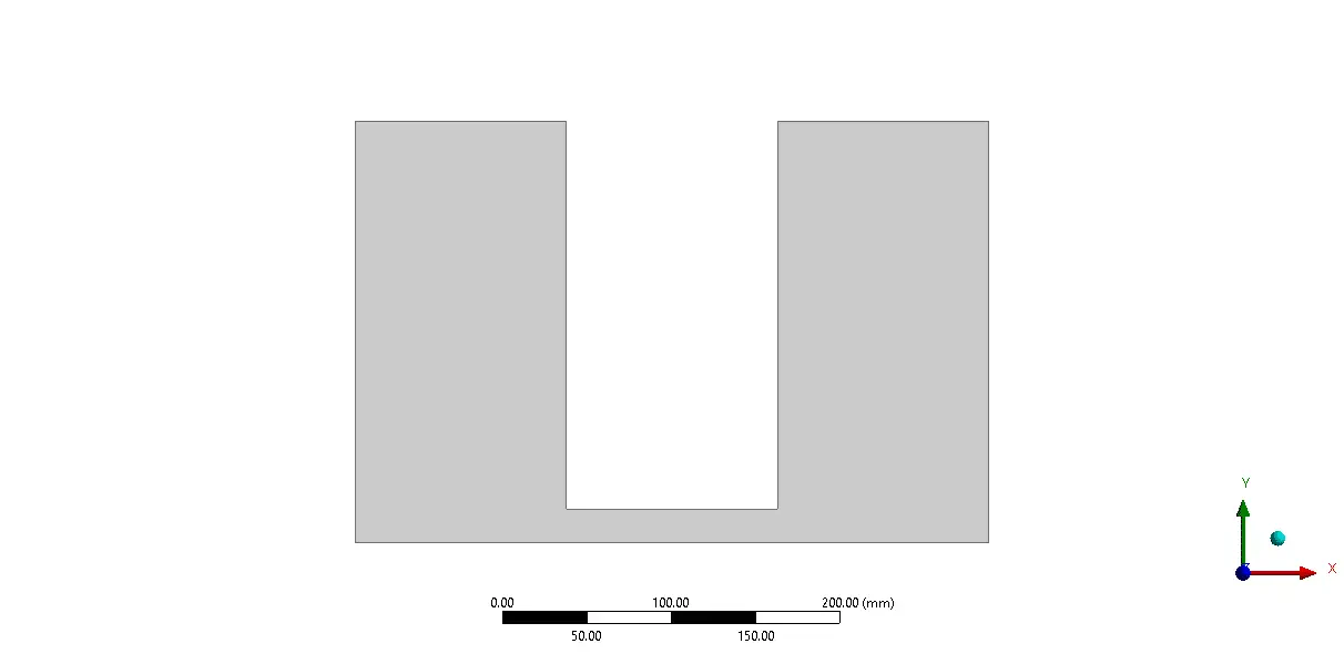
The geometry of the solution consisted of two reservoirs that Each of them has dimensioned 1.25*2.5 m. The 2D geometry of this project has been produced with Ansys Design Modeler software.
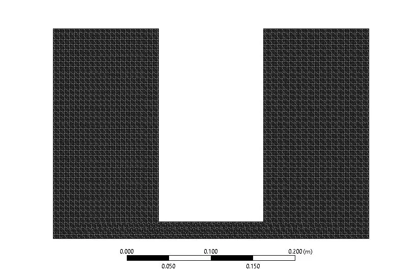
Mesh is created with Ansys meshing software, and the mesh type is structured. The number of cells is 32510.
Tank Charge CFD Simulation
We consider several assumptions to simulate the present model:
- Due to the incompressibility of the flow, the pressure-based solver method has been selected.
- The simulation is transient.
- The gravity effect is considered equal to -9.81 m.s-2on Y-axis
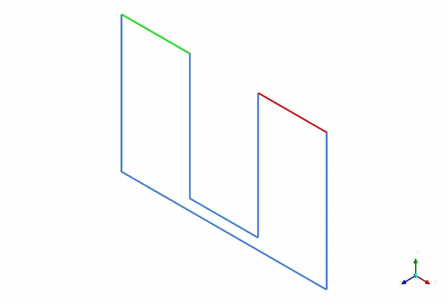
In the figure below, taken from Ansys CFD-post software, the red lines are related to temperatures. The blue lines are adiabatic, and the blue and orange lines are related to heat1 and wall. The type of walls, inlet vent, and outlet vent boundary conditions Also shown in blue, green, and red respectively a wall, inlet vent, and outlet vent.
The following tables represent a summary of the defining steps of the problem in this project and its solution.
Multiphase | Model | Volume of Fluid |
Number of Eulerian phases | 2(air & water) | |
Interface modeling | Sharp | |
Formulation | implicit | |
Primary phase | air | |
Secondary phase | Water | |
Viscous | k-epsilon | Realizable |
Near wall treatment | Standard wall functions | |
Material Properties | ||
Air | Density | 1.225 |
viscosity | 1.7894e-05 | |
| water-liquid | Density | 998.2 |
viscosity | 0.001003 | |
| Boundary conditions | ||
Walls | wall | |
Wall motion | Stationary wall | |
Inlet-vent | Inlet-vent | |
gauge pressure | 0 pascal | |
outlet-vent | outlet-vent | |
gauge pressure | 0 pascal | |
Pressure profile multipier | 1 | |
| Solution Methods | ||
Pressure-velocity coupling | couple | |
Spatial discretization | Pressure | presto |
momentum | second-order | |
Volume fraction | Compressive | |
Turbulent kinetic energy | First-order upwind | |
Turbulent dissipation rate | First-order upwind | |
Initialization | ||
Initialization method | Standard | |
Patch | Phase | water |
Variable | Volume Fraction | |
Zones to patch | Surface-body | |
value | 1 | |
Run calculation | ||
Time step size | 0.001 | |
Max iterations/time step | 20 | |
Number of time steps | 10000 | |
This simulation presents two-dimensional contours related to volume fraction, pressure, velocity, and turbulent kinetic energy. Also, as the attached animation shows, the air phase moves upwards by moving the water fluid towards the tank containing air. We observe After a few seconds and according to the law of hydrostatic pressure, the pressure is equal at the same heights.