Description

This product is validation of simulating a wall trombe based on the paper "The thermal performances of a solar wall "by ANSYS Fluent software.

A passive solar architectural element known as a trombe wall, is a thick, black-painted wall that faces south (or north, depending on the hemisphere) and is composed of a heat-absorbing material like stone or concrete. Glass or clear plastic coverings are placed a few inches apart from the wall. Solar energy is captured and stored in part by this arrangement.
The Trombe wall operates on the basic principles of solar energy heat transfer: absorption, conduction, and convection.

The 2-D geometry of this project is drawn in Design Modeler and meshed in ANSYS Meshing producing 26,550  structured elements.

Methodology

This simulation is done transiently by considering y direction gravity. As the absorber is exposed to a volumetric heat flux, we defined a  heat source in the cell zone condition for absorber domain using UDF. The heat flux is defined in the following:

source heat flux = 55000*sin(3.14159265*time/36000)

The time step size is 1[s] and the number of time step is 86,400.

Conclusion

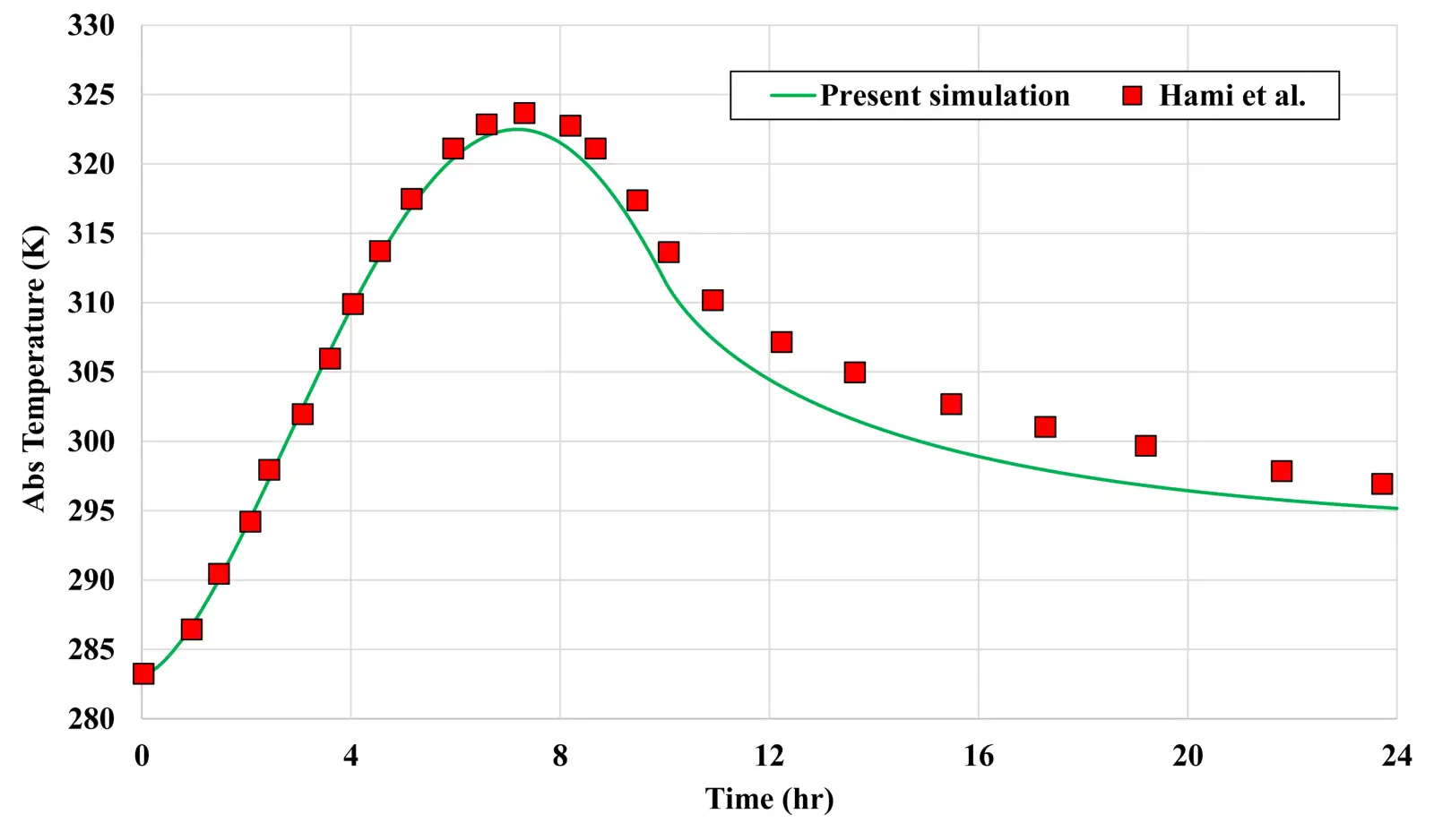
As shown in the figure below, the temperature of the absorber obtained from the simulation is compared with the numerical results of Mr. Hami et al. As can be seen in this figure, there is a good accuracy between the results, of course, in the areas before the temperature peak, the results are almost identical, and after the temperature peak, there is a slight difference between the results. The biggest difference in the temperature of the absorber after 13 hours from the start of the simulation was 1.2%, which can be said to be insignificant and acceptable.

Also the contours of temperature and velocity are presented in the 6, 12 and 18 hours from the beginning of the simulation.