
Progress to Intermediate ANSYS Fluent Skills
Price: $29
The final stage of MR CFD's three-course path — for users who already mesh, run transient cases, and read their own residuals, and now want to solve the problems that defeat most CFD engineers.
Master the hard end of Fluent: custom solver behavior with UDFs, two-way FSI, dynamic and moving mesh, rotating machinery (MRF/SRF, multistage compressors), high-speed and reacting flows (supersonic shocks, scramjet combustion), and advanced multiphysics (MHD/EHD, FW-H acoustics, cavitation, PCM, Eulerian multiphase).
Built for real workflows: run large transient cases on MR CFD's HPC, use AI as an accelerator where it genuinely helps, and earn a path into the internship program to apply these skills on live consulting projects.
Urban Planning: Pollution of a Street between Buildings
DescriptionThis project uses ANSYS Fluent to simulate air pollutant dispersion in a street canyon between buildings, applying species transport modeling to a core urban planning and environmental engineering problem. Building geometry strongly influences how pollutants accumulate or disperse in urban street canyons, making this analysis relevant to air quality management and sustainable city design.MethodologyA 3D street canyon and building geometry is built in DesignModeler and meshed in ANSYS Meshing using a structured grid of 274,496 elements. The simulation uses a pressure-based, steady-state, incompressible solver, with the Species Transport model configured to track pollutant dispersion. Gravitational effects and appropriate boundary conditions are applied to represent realistic urban airflow.ConclusionResults include pressure, velocity, and pollutant concentration contours, characterizing how airflow patterns between buildings drive pollutant accumulation or dispersion. The analysis evaluates pollutant concentration at different locations within the urban setting, revealing how street canyon geometry and building configuration affect local air circulation and air quality — insights relevant to urban planning, traffic emissions assessment, and sustainable city design.
Progress to Intermediate ANSYS Fluent Skills
Price: $29
The final stage of MR CFD's three-course path — for users who already mesh, run transient cases, and read their own residuals, and now want to solve the problems that defeat most CFD engineers.
Master the hard end of Fluent: custom solver behavior with UDFs, two-way FSI, dynamic and moving mesh, rotating machinery (MRF/SRF, multistage compressors), high-speed and reacting flows (supersonic shocks, scramjet combustion), and advanced multiphysics (MHD/EHD, FW-H acoustics, cavitation, PCM, Eulerian multiphase).
Built for real workflows: run large transient cases on MR CFD's HPC, use AI as an accelerator where it genuinely helps, and earn a path into the internship program to apply these skills on live consulting projects.
-
Section 1
Engineering Fields
$18-
This project simulates film cooling on a gas turbine blade — the technique that lets turbine blades survive gas temperatures well above their material limits by holding a thin layer of cool air against the surface. The cooling air, bled from the compressor stage, is fed through internal channels and ejected through discrete holes to form a protective film over the blade.The study is set up as a conjugate heat transfer (CHT) problem: the fluid domain (hot gas and cooling air) and the solid blade are coupled at the walls, so heat conducts through the blade while the external hot gas and the internal/film cooling air exchange heat with it simultaneously. Turbulence is modeled with k-ω SST, which resolves both the near-wall film behavior and the free-stream mixing between cool and hot streams.Geometry is built in Design Modeler, meshed in ANSYS Meshing, then converted to a polyhedral mesh (~2.7 million cells) in ANSYS Fluent for better gradient resolution and faster convergence around the cooling holes.What the results show: pathlines trace the cooling air through the blade's internal channels and out through the film holes, where it forms a thin thermal barrier over the surface. Film thickness varies along the blade — thickest near the holes — and the film is turbulent, mixing with the hot gas downstream and progressively losing effectiveness. The simulation makes the core design trade-off visible: hole size, shape, spacing, count, and injection angle all control how well the film holds before the hot gas entrains it.You'll learn to: set up a coupled fluid–solid CHT model, mesh and inject through discrete cooling holes, choose and justify k-ω SST for film flows, and read film effectiveness from temperature fields and pathlines.
Lesson 1 32m 42s -
This project simulates a greenhouse roof watering system — water sprayed from roof-mounted nozzles falling through air and accumulating on the surface below. It's a clean introduction to two-phase flow under gravity, where the goal is to track where the water goes and how it distributes once it leaves the nozzle.The case is built as a 2-D transient model in Design Modeler, with the domain split into two sections: a resident pool of water at the bottom and an upper region carrying a velocity inlet and an outlet. The tank sides are treated as walls. Meshing is done in ANSYS Meshing (~208,921 elements).Physics is handled with the Eulerian multiphase model, using air as the primary phase and water as the secondary phase. Water enters at 0.3 m/s with gravity acting at −9.81 m/s² on the y-axis, and turbulence is closed with the SST k-ω model. Because the spray develops over time — water pumping out, falling, and pooling — the solver is run transient.What the results show: velocity fields and air/water volume-fraction contours capture the full sequence — water pumping through the roof nozzles, dropping under gravity, and spreading across the bottom surface. The volume-fraction field is the key output: it shows coverage and where water collects, which is exactly what you'd tune in a real irrigation layout.You'll learn to: set up a 2-D transient Eulerian two-phase case, define primary/secondary phases, apply gravity correctly, and read phase distribution from volume-fraction contours.
Lesson 2 10m 56s -
DescriptionThis project simulates airflow within a building’s double-skin façade (DSF) using ANSYS Fluent. In a DSF, solar-heated air rises due to buoyancy, providing passive heating and aiding ventilation/cooling inside the building.The 3D geometry (DesignModeler) is a rectangular cavity measuring 0.6 × 3.2 × 5 m, composed of a duct for airflow and a glazed section that absorbs solar heat. Openings include a 0.2 m rectangular inlet at the bottom of the glass wall and a 0.2 m outlet near the top. Meshing (ANSYS Meshing) yields 490,725 elements.MethodologyThe study evaluates buoyancy-driven circulation in the DSF cavity. The glass section is modeled with a volumetric heat generation of 6940 W/m³ to represent solar gain. Building walls are brick and subject to convection to the interior: T = 300 K, h = 23 W/m²·K (free convection).Supply air enters the façade at 304.55 K and atmospheric pressure. To capture buoyancy, air density follows the ideal gas law, and gravity = 9.81 m/s² is applied.ConclusionPost-processing provides 2D/3D pressure, velocity, and temperature contours, plus 2D/3D velocity vectors. The vectors show an upward flow in the cavity, confirming buoyancy-driven ventilation within the double-skin façade.
Lesson 3 17m 15s -
DescriptionThis project simulates the delivery of an asthma spray into human lungs using ANSYS Fluent. The 3D geometry—built in SpaceClaim—represents a simplified lung model with a 50 cm inlet diameter. The mesh (ANSYS Meshing) contains 3,734,238 elements. Given the time-dependent nature of inhalation and particle motion, a transient solver is used.Asthma Spray MethodologyA one-way coupled Discrete Phase Model (DPM) tracks aerosol particles moving through a continuous air phase. Air enters at 5 m/s, with gravity set to −9.81 m/s² along the z-axis. Particles (diameter 100 µm) are introduced via a surface-velocity injection at the inlet. Turbulence is resolved with the realizable k–ε model. Particle trajectories inside the lung domain are computed and visualized to assess transport and deposition behavior.ConclusionPost-processing provides 2D and 3D contours of velocity and pressure, along with an animation of particle tracks throughout the lungs, illustrating the spray’s distribution following inhalation.
Lesson 4 15m 41s -
This project simulates a water spray issuing from a small circular inlet into a larger cubic enclosure, tracking the behavior of the spray particle by particle. It's the standard introduction to the Discrete Phase Model (DPM) — the Lagrangian approach Fluent uses when you care about the trajectory, velocity, and dispersion of individual droplets rather than a continuous second phase.The geometry is a rectangular cube with a circular inlet on the top wall, built in Design Modeler and meshed in ANSYS Meshing with an unstructured mesh (25,464 cells). Because droplets move discretely through a continuous medium, the case is solved with a Lagrangian DPM layered on the continuous (Eulerian) air flow, and run transient to capture how the spray develops in time.The key setup step is defining the injection: water is released as a surface injection from the inlet, with the droplets treated as inert particles. This is where DPM differs from a multiphase model — you specify how, where, and at what size/velocity the particles enter, and Fluent integrates each trajectory through the flow field.What the results show: velocity and mass-concentration contours of the water particles at the final time step, plus 3-D particle tracks colored by particle speed and droplet diameter. The tracks confirm the injection is set up correctly — droplets disperse discretely from the top inlet and distribute through the enclosure, which is exactly the behavior you'd analyze when sizing nozzles or predicting coverage.You'll learn to: distinguish DPM (Lagrangian) from Eulerian multiphase, define a surface injection of inert particles, couple the discrete phase to a transient continuous flow, and read spray behavior from particle tracks and concentration contours.
Lesson 5 21m 22s -
This project simulates heat extraction from a geothermal reservoir using a single U-tube Downhole Heat Exchanger (DHE) — a U-shaped pipe set in a wellbore through which a working fluid circulates to draw heat out of the ground. It's a strong study in natural-convection-driven conjugate heat transfer, where the heat path runs from the surrounding ground, through the borehole fluid, and into the circulating tube water.The model is built from three coupled parts — the U-tube, the borehole, and the ambient geothermal reservoir — and is a scaled version of a real field case (which sits ~200 m underground). Here the ground zone and U-tube are scaled to 6 m and 3.2 m depth, with a 0.0875 m tube diameter inside a 0.35 m borehole, all within a 3 m ground cylinder. Geometry is built in Design Modeler and meshed in ANSYS Meshing as a polyhedral mesh (~1.75 million cells).The physics centers on free (natural) convection: the solid ground temperature is set as a linear function of depth using a Named Expression, so the borehole heats from the bottom up. Gravity is enabled, and water's thermal conductivity and heat capacity are defined as temperature-dependent via the polynomial method — the buoyancy that drives the whole problem depends on getting these property variations right. Turbulence uses the Realizable k-ε model with standard wall functions, and the flow is solved steady.What the results show: temperature and pressure contours plus velocity vectors for both the tube and borehole zones. Convective heat transfer raises the tube outlet temperature to 305.47 K. The velocity vectors reveal the mechanism clearly — a vortex forms at the bottom of the hole, intensifying turbulence and heat transfer; water near the hot wall warms, loses density, and rises, then cools and sinks, completing the natural-convection loop that feeds heat into the tube.You'll learn to: set up buoyancy-driven natural convection, define depth-dependent solid temperatures with Named Expressions, model temperature-dependent fluid properties, and run a coupled solid–fluid heat exchange case.
Lesson 6 19m 46s -
Battery CFD Simulation Concepts in ANSYS Fluent: A Comprehensive OverviewWelcome to the 2nd chapter of our Battery Training Course. In this training video, we describe the Battery Model Concepts in ANSYS Fluent software. We provide you with a detailed and comprehensive tutorial; so that you will master all concepts of the battery model without any problems.Introduction to BatteryIn the first step, we present a general introduction to the battery. This introduction provides a basis for using the battery model in ANSYS Fluent.Battery MechanismBattery Geometry DefinitionSingle Battery and Battery PackFundamental Battery ConceptsIn the next step, we discuss battery concepts in ANSYS Fluent software. We provide the different solution methods of the battery model and corresponding formulations; so that you could set up the battery model settings with advanced knowledge.Battery Solution MethodsFor example, we introduce different solution methods for coupling thermal and electrochemical behaviors. We describe these solution methods comprehensively and study the related governing equations.CHT Coupling MethodFMU-CHT Coupling MethodCircuit Network Solution MethodMSMD Solution Method (Multi-Scale Multi-Domain)Battery electrochemistry modelsIn the solution methods, potential and energy equations are solved in ANSYS Fluent. We introduce different electrochemical models for computing the source terms in equations such as the current transfer and heat generation rate.NTGK ModelEquivalent Circuit Model (ECM)Newman P2D ModelIn different electrochemical models, we explain all relations and the corresponding coefficients. Then, we refer to the model parameters and their dependence on DoD (depth of discharge) and SoC (State of Charge).Battery Pack definitionAfter an introduction to electrochemical models, we focus on the computational domain of the model. So, we define battery cell, battery module, and battery pack. We mention the comparison between parallel and series connections, and the nPmS pattern arrangement.Then, we introduce the different types of connections in battery packs.Real ConnectionsVirtual Connections (Tab Surface Based and Active Zone Volume Based)Battery Advanced OptionsIn addition, we mention a series of optional capabilities and tools in battery modeling.Thermal Abuse ModelBattery Life Model (Cycle Life Loss and Calender Life Loss)Pack Builder ModelBattery Model Settings in ANSYS FluentIn the final step, we discuss the battery model settings in ANSYS Fluent. We review all the steps necessary for a battery simulation process.so, we explain all settings tabs of the battery model in ANSYS Fluent.ّModel OptionsConductive ZonesElectric ContactsModel ParametersAdvanced OptionsIn battery simulation, we specify the operating conditions during the battery charging/discharging. Hence, we can use different electrical parameters.C-rateCurrentVoltagePowerResistanceProfile (Time-Schedules and Event-Scheduled)Why This Episode Is Crucial for Your Battery CFD JourneyThis foundational episode equips you with:A comprehensive understanding of battery principlesInsight into ANSYS Fluent’s capabilities for battery simulationPractical knowledge of setting up various electrochemistry modelsBy mastering these concepts, you’ll be well-prepared to tackle more advanced battery simulations in subsequent chapters of the course.Target AudienceThis episode is ideal for:Beginners in battery CFD simulationExperienced CFD users new to battery modelingResearchers and engineers looking to refresh their battery simulation fundamentalsLearning OutcomesAfter completing this episode, you will:Understand the core principles of battery cell and battery packBe familiar with ANSYS Fluent’s battery modeling capabilitiesKnow how to set up different solution methods and electrochemistry models in ANSYS FluentBe prepared for more advanced battery simulations in future episodesEmbark on your electrolysis CFD simulation journey with this comprehensive introduction, setting a strong foundation for the exciting chapters ahead!
Lesson 7 58m 19s -
Tank Discharge System CFD Analysis - ANSYS Fluent SimulationProject OverviewThis computational fluid dynamics study investigates gravitational water discharge from a multi-tank system using ANSYS Fluent software. The simulation employs the Volume of Fluid (VOF) model to accurately capture the two-phase flow dynamics involving water and air phases throughout the interconnected tank network.System ConfigurationMulti-Tank ArrangementThe computational domain encompasses three interconnected storage tanks connected through a piping network. The primary tank features rectangular geometry with dimensions of 229.4 mm by 157.7 mm, designed to serve as the initial water reservoir. The secondary tank utilizes an octagonal configuration with uniform side lengths of 51.3 mm, providing intermediate storage capacity. The tertiary tank employs rectangular geometry measuring 229.4 mm by 100 mm, functioning as the final collection vessel.Geometric Design and Computational GridTwo-Dimensional Model DevelopmentThe geometric configuration was developed using Design Modeler software, incorporating realistic tank geometries and interconnecting pipe networks to simulate industrial discharge systems. The design includes air circulation pathways to maintain atmospheric pressure balance during discharge operations.Mesh Generation SpecificationsThe computational grid was generated using ANSYS Meshing software with an unstructured mesh topology containing 15,310 elements. This mesh density provides adequate resolution for capturing the complex free surface dynamics and flow transitions between the interconnected tank systems.CFD Simulation ConfigurationFundamental Modeling AssumptionsThe simulation utilizes a pressure-based solver approach suitable for incompressible flow conditions. The analysis is conducted in transient mode to capture the temporal evolution of the discharge process and free surface movement. Gravitational acceleration of -9.81 m/s² is applied along the negative y-axis to drive the discharge phenomenon.Multiphase Flow ModelingThe Volume of Fluid homogeneous model governs the two-phase flow field equations with air and water as the defined Eulerian phases. Sharp interface modeling with interfacial anti-diffusion capabilities ensures accurate free surface tracking throughout the discharge process. The implicit formulation with implicit body force treatment provides robust solution stability for gravitational flow applications.Viscous Flow TreatmentLaminar viscous modeling is employed to solve the flow field equations, appropriate for the low Reynolds number conditions typical in gravitational discharge applications. This approach provides accurate representation of viscous effects without the computational overhead of turbulence modeling.Material PropertiesAir properties are defined with density of 1.225 kg/m³ and dynamic viscosity of 1.7894×10⁻⁵ Pa·s, representing standard atmospheric conditions. Water-liquid properties utilize density of 998.2 kg/m³ and dynamic viscosity of 0.001003 Pa·s, corresponding to water at standard temperature conditions.Numerical Solution MethodsThe pressure-velocity coupling employs the SIMPLE algorithm for iterative solution convergence. Pressure discretization utilizes the PRESTO! scheme, optimized for complex geometries with significant density variations. Momentum equations are solved using second-order upwind discretization for enhanced accuracy, while volume fraction transport employs the compressive scheme to maintain sharp interface definition.Domain Initialization and PatchingStandard initialization is applied throughout the computational domain with subsequent patching operations to establish initial water distribution. The primary tank region is initialized with unity volume fraction for the water phase, corresponding to coordinates spanning from x = 0.08 m to x = 0.379 m and y = 0.2264246 m to y = 0.33 m.Temporal Solution ConfigurationThe simulation employs adaptive time advancement with initial time step size of 1×10⁻⁵ seconds. The adaptive scheme maintains minimum time step of 1×10⁻⁵ seconds and maximum time step of 0.001 seconds, with total execution of 10,000 time steps to capture complete discharge dynamics.Results and Flow AnalysisDischarge Process CharacterizationThe simulation results present comprehensive visualization of volume fraction distribution, pressure fields, velocity magnitude, and streamline patterns throughout the discharge evolution. The analysis demonstrates progressive water transfer from the primary tank to the secondary tank, with subsequent overflow to the tertiary tank as storage capacity limitations are exceeded.Free Surface DynamicsVolume fraction contours clearly illustrate the free surface evolution and interface tracking accuracy throughout the discharge process. The VOF model successfully captures the complex interface deformation as water flows through the connecting pipes and fills the downstream tanks.Flow Field AnalysisVelocity and streamline visualizations reveal the flow patterns within each tank and connecting pipe network. The results demonstrate the influence of air circulation pathways in maintaining pressure equilibrium and preventing vacuum formation during discharge operations.Engineering InsightsThe simulation provides valuable insights into multi-tank discharge system design, including optimal pipe sizing, tank geometry effects, and air circulation requirements. The pressure distribution analysis enables assessment of system efficiency and identification of potential flow restrictions or optimization opportunities.
Lesson 8 20m 35s -
Mastering Brake Disk Heat Transfer: A Beginner's Guide to Automotive Thermal CFD SimulationWelcome to the “Brake Disk Heat Transfer CFD Simulation” episode of our “THERMAL Engineers: BEGINNER” course. This comprehensive module introduces you to the critical world of automotive thermal management, focusing on the complex heat transfer mechanisms in high-performance braking systems using ANSYS Fluent. Dive into this essential aspect of vehicle safety and performance, and learn how to optimize brake disk cooling efficiency through powerful CFD techniques.Understanding Heat Generation and Dissipation in Brake DisksBefore delving into the simulation specifics, we’ll explore the fundamental concepts of heat transfer in brake systems.Friction-Induced Heat GenerationDiscover the physics behind heat generation during braking events and its impact on brake disk performance.Heat Dissipation Mechanisms in Brake SystemsLearn about the various ways heat is dissipated from brake disks, including convection, conduction, and radiation.Analyzing Transient Heat Transfer During Braking EventsThis section focuses on the dynamic nature of heat transfer in brake disks during operation:Thermal Cycling and Its EffectsGain insights into how repeated heating and cooling cycles affect brake disk material properties and performance.Thermal Stress DevelopmentUnderstand how temperature gradients within the brake disk lead to thermal stresses and potential failure modes.Evaluating Cooling Efficiency of Brake Disk DesignsDive into the specifics of modeling and analyzing cooling performance in brake disks:Vented vs. Solid Disk DesignsExplore the differences in heat dissipation capabilities between vented and solid brake disk designs.Surface Area Optimization for CoolingLearn how different surface features and patterns influence the overall cooling efficiency of brake disks.Setting Up the Brake Disk Simulation EnvironmentIn this section, we’ll guide you through the process of preparing your CFD simulation for brake disk analysis:Geometry Preparation and ImportationMaster the basics of working with pre-designed brake disk geometries in ANSYS Fluent, ensuring proper setup for accurate simulation.Mesh Generation Strategies for Brake Disk ModelsLearn techniques for creating appropriate meshes that capture both solid and fluid domains effectively, crucial for precise results.Defining Boundary Conditions for Brake Disk Heat TransferUnderstand the essential parameters required for simulating brake disk performance:Friction Heat Source DefinitionGain insights into setting up realistic heat generation conditions that mimic actual braking scenarios.Ambient Conditions and Cooling Air PropertiesLearn to define appropriate boundary conditions for the surrounding air, including temperature, pressure, and velocity parameters.Configuring Heat Transfer Models for Accurate SimulationDevelop skills in setting up the necessary models for comprehensive brake disk analysis:Selecting Appropriate Turbulence ModelsUnderstand how to choose and configure turbulence models suitable for the complex air flow around rotating brake disks.Implementing Radiative Heat Transfer SettingsLearn to activate and set up radiative heat transfer models that accurately represent heat dissipation from hot brake surfaces.Analyzing Simulation Results for Brake Disk PerformanceMaster the interpretation of CFD simulation outcomes:Visualizing Temperature DistributionsDevelop techniques for creating and interpreting temperature contours across the brake disk during and after braking events.Evaluating Thermal GradientsLearn to generate and analyze thermal gradient maps to assess potential areas of thermal stress and fatigue.Assessing Brake Disk Cooling EffectivenessLearn to evaluate the overall performance of your simulated brake disk:Calculating Heat Dissipation RatesDiscover methods for computing the rate of heat dissipation from the brake disk under various operating conditions.Identifying Hotspots and Cooling InefficienciesDevelop skills in recognizing areas of inefficient heat dissipation and propose improvements to the brake disk design.Practical Applications and Industry RelevanceConnect simulation insights to real-world engineering challenges:Optimizing Brake Disk Designs for High-Performance VehiclesExplore how CFD simulations can inform better brake disk designs for racing and high-performance automotive applications.Thermal Management in Heavy-Duty Braking SystemsUnderstand the role of brake disk analysis in developing efficient cooling solutions for trucks, buses, and industrial vehicles.Why This Module is Essential for Beginner Thermal EngineersThis beginner-friendly module offers a practical introduction to brake disk CFD simulation, a critical skill in modern automotive and mechanical engineering. By completing this simulation, you’ll gain valuable insights into:Fundamental principles of friction-induced heat transfer and dissipationBasic CFD techniques for modeling transient thermal events in rotating componentsPractical applications of CFD analysis in optimizing safety-critical automotive systemsBy the end of this episode, you’ll have developed essential skills in:Setting up and running basic brake disk simulations in ANSYS FluentInterpreting simulation results to assess thermal performance and identify potential issuesApplying CFD insights to improve thermal management strategies in braking systemsThis knowledge forms a crucial foundation for aspiring thermal engineers, providing a springboard for more advanced studies in automotive thermal management, safety system design, and thermal analysis of high-stress mechanical components.Join us on this exciting journey into the world of brake disk CFD simulation, and take your first steps towards becoming a proficient thermal engineer in the rapidly evolving field of automotive and mechanical system thermal management!
Lesson 9 12m 9s -
DescriptionThis project models heat transfer from a wall-mounted radiator inside a room using ANSYS Fluent. The heater, attached to one sidewall, acts as a heat source with a constant heat flux of 1886.792 W/m². The sidewalls and ceiling are 0.2 m thick wood and exchange heat with the outdoors via convection (ambient 280 K, h = 10 W/m²·K). The study focuses on natural convection and buoyancy-driven flow inside the room, so gravity is included.The 3D geometry is created in SpaceClaim. Meshing is performed in ANSYS Meshing with a structured grid totaling 87,865 elements.MethodologyThe energy model is enabled to resolve conjugate heat transfer between the heater and room air, capturing buoyancy-induced circulation.ConclusionPost-processing yields 2D and 3D contours of velocity, temperature, and pressure, along with pathlines and velocity vectors. Results show the radiator elevates room air temperature, with the strongest heating and velocity increases near the walls, especially in the vicinity of the heater.
Lesson 10 17m 11s -
DescriptionThis project uses ANSYS Fluent to simulate counterflow in a canal and analyze the resulting fluid behavior. The setup features a main water stream moving along the canal while a second stream is injected in the opposite direction from a floor-mounted pipe.The 3D geometry (DesignModeler) represents a straight channel 8 m long with a 3 m × 1 m rectangular cross-section. A 4 m long pipe of 0.05 m diameter lies along the canal floor. Meshing (ANSYS Meshing) yields 256,899 elements. A transient solver is used.Counterflow MethodologyThe main channel inflow velocity is 0.3 m/s, while the pipe issues flow at 2 m/s in the opposite direction. The region above the water surface is open to air; a pressure inlet boundary with 0 Pa gauge represents ambient conditions.Because both water and air are present, a VOF multiphase model is employed, with the standard k–ε model for turbulence.ConclusionPost-processing provides 2D and 3D fields of pressure, velocity, and phase volume fraction for water and air. The opposing jet perturbs the free surface and entrains air, producing zones with a locally reduced water volume fraction where the counterflow interacts with the main stream.
Lesson 11 12m 6s -
What You'll BuildThis lesson walks you through a CFD simulation of short waves on the sea surface — a fundamental problem in coastal, marine, and offshore engineering. Using ANSYS Fluent's ability to generate waves directly at a boundary, you'll create a realistic propagating wave field and track how the air–water interface evolves over time, all based on First-Order Airy (linear) wave theory.This is your introduction to wave generation in CFD, a capability that underpins the design of breakwaters, offshore platforms, ships, and coastal structures.What You'll LearnThe basics of First-Order Airy wave theory and how it's applied inside FluentHow to design a 2-D sea domain (210 cm long × 76 cm high) in SpaceClaimHow to generate an unstructured mesh (~55,000 cells) suited to free-surface wave trackingHow to set up the VOF multiphase model with air and water phases, sharp interface modeling, and explicit formulation with implicit body forceHow to apply the open-channel wave boundary condition to send waves into the domain from the inletWhy a transient, pressure-based solver with the laminar viscous model is appropriate for this wave problemHow to configure adaptive time stepping for stable, efficient wave propagationHow to use PRESTO! pressure discretization and Compressive volume-fraction discretization to keep the interface sharpHow to patch the initial water region and post-process velocity contours, observing how moving waves induce vortices and turbulence in the air above the surfaceWhy It MattersWave modeling is essential across naval architecture, coastal protection, renewable wave energy, and offshore oil and gas. The open-channel wave boundary condition you master here is the gateway to simulating realistic ocean environments — from ship seakeeping to wave-structure interaction.
Lesson 12 15m 35s -
Mastering the Discrete Phase Model (DPM) in ANSYS FLUENT: A Comprehensive GuideDive deep into the heart of multiphase flow simulations with our second episode of the “DPM: All Levels” course. This comprehensive tutorial unlocks the full potential of the Discrete Phase Model (DPM) module in ANSYS FLUENT, equipping you with the knowledge to tackle complex particle-laden flow problems with confidence.Episode OverviewIn this extensive exploration of ANSYS FLUENT’s DPM capabilities, you’ll gain hands-on experience navigating the software’s interface and mastering its diverse features. From basic settings to advanced modeling techniques, this episode covers it all, ensuring you’re well-prepared to implement DPM in your simulations effectively.Key Learning Objectives1. DPM Dialog Box Mastery- Navigate the Discrete Phase Model Dialog Box with ease - Understand interaction settings and particle treatment options - Master tracking parameters for precise simulations2. Advanced Physical Models- Explore a wide range of physical phenomena, including: - Particle Radiation Interaction - Thermophoretic and Saffman Lift forces - Virtual mass and Pressure gradient forces - Erosion/Accretion modeling - Temperature-dependent effects - Two-way turbulence coupling - Collision and breakup models3. Injection Techniques- Learn various injection types: Single, Group, Surface, and Cone - Understand different particle types: Massless, Inert, Droplet, Combusting, and Multi-component - Master diameter distribution methods for realistic particle populations4. Drag Laws and Breakup Models- Implement appropriate drag laws for your specific applications - Understand and apply breakup models for complex multiphase flows5. Turbulent Dispersion and Boundary Conditions- Grasp the concepts of Stochastic tracking and Cloud tracking - Master DPM boundary conditions for accurate particle-wall interactionsWhy This Episode Is EssentialAs the cornerstone of our DPM course, this episode provides:In-depth understanding of ANSYS FLUENT’s DPM interfacePractical skills to set up and customize DPM simulationsKnowledge to choose appropriate models for your specific engineering problemsFoundation for advanced DPM applications covered in later episodesWho Should WatchThis episode is invaluable for:CFD engineers looking to expand their multiphase modeling capabilitiesResearchers working on particle-laden flows in various industriesANSYS FLUENT users aiming to leverage DPM for complex simulationsStudents and professionals seeking to enhance their CFD skillsetElevate Your DPM Expertise with ANSYS FLUENTDon’t miss this opportunity to become proficient in one of the most powerful tools for multiphase flow simulations. Whether you’re simulating sprays, particle transport, or erosion phenomena, the skills you’ll gain in this episode are essential for accurate and efficient DPM modeling.What's Next?After mastering the ANSYS FLUENT DPM interface, you’ll be well-prepared to tackle the practical applications covered in subsequent episodes, including:Spray simulations with evaporation and breakupWet combustion modelingErosion analysis in complex geometriesRespiratory disease transmission studiesEnroll now and take a significant step towards becoming a DPM expert. Transform your approach to multiphase flow simulations and unlock new possibilities in your engineering and research projects!
Lesson 13 47m 9s -
This project simulates the airflow and heat transfer inside a Heller-type dry cooling tower — the indirect cooling system used in thermal power plants to reject heat from the working fluid (water) to ambient air without evaporative water loss. After leaving the condensers, the hot water is pumped through a ring of air-cooled heat exchangers; the tower draws cooling air through them by natural draft, created by the density difference between the warm air inside the tower and the cooler air outside.The study captures the core physics that governs tower performance: the temperature driving force. The larger the gap between the working fluid and ambient air, the stronger the natural draft and the better the cooling. This is also why these towers lose efficiency in summer — as ambient temperature rises, the driving force shrinks, forcing the plant to cut power output and increase water consumption to maintain cooling. The simulation lets you see and quantify that buoyancy-driven flow directly.Geometry & mesh: the model includes the cooling tower, the heat-exchanger (radiator) ring, the flow domain, and the air inlet, built and meshed in GAMBIT with an unstructured mesh of 1,343,988 cells.Setup: the case is solved steady with a pressure-based solver, with gravity enabled at −9.81 m/s² in the Y direction — essential, since the natural draft is entirely buoyancy-driven. Turbulence uses the standard k-ε model with standard wall functions, and the energy equation is on.Boundary conditions reproduce the natural-draft setup:Inlet: pressure inlet, 0 Pa gauge total pressure, normal to boundaryOutlet: pressure outlet, 0 Pa gauge, backflow temperature 303 KRadiator (heat exchanger): modeled as a heated surface at 318 K with a heat generation rate of 14,861.52 W/m³, and its shadow face at 313 KWalls: stationary, zero heat fluxSolution uses SIMPLE pressure–velocity coupling with first-order upwind discretization for momentum, energy, and turbulence (standard scheme for pressure and density), and standard initialization at 303 K.What the results show: contours of velocity, pressure, and temperature, along with flow streamlines through the tower. Together they reveal how air is drawn in through the heat exchangers, heats up, and rises through the tower — and how the temperature field across the radiator ring sets the cooling capacity available to the plant.You'll learn to: set up a buoyancy-driven natural-draft flow, represent a heat-exchanger ring with a heated radiator surface and heat generation rate, configure a steady pressure-based solver with the energy equation, and interpret cooling-tower performance from temperature and streamline fields.
Lesson 14 14m 43s -
DescriptionThis module covers multistage compressor simulation using CFD, applying rotary equipment and turbomachinery modeling principles to a compressor configuration with two rotor and two stator rows. Multistage compressors are widely used across mechanical engineering applications, including gas turbines, HVAC systems, and process industries, making this a foundational skill for turbomachinery-focused CFD work.MethodologyThe simulation setup covers configuring rotating reference frames for the rotor stages, defining interface conditions between rotor and stator domains, and applying turbulence models suited to compressor flow. Boundary conditions specific to compressor operation are established, and the simulation is run with convergence monitored throughout the solution process.ConclusionThe analysis examines flow patterns, pressure ratios, and temperature changes across the compressor stages, visualized through velocity fields, pressure distributions, and streamlines. This understanding supports the analysis and optimization of compression systems such as gas turbine engines, industrial air compressors, and refrigeration systems, and builds core skills for tackling advanced turbomachinery problems in mechanical engineering.
Lesson 15 14m 43s -
DescriptionThis project uses ANSYS Fluent to simulate air pollutant dispersion in a street canyon between buildings, applying species transport modeling to a core urban planning and environmental engineering problem. Building geometry strongly influences how pollutants accumulate or disperse in urban street canyons, making this analysis relevant to air quality management and sustainable city design.MethodologyA 3D street canyon and building geometry is built in DesignModeler and meshed in ANSYS Meshing using a structured grid of 274,496 elements. The simulation uses a pressure-based, steady-state, incompressible solver, with the Species Transport model configured to track pollutant dispersion. Gravitational effects and appropriate boundary conditions are applied to represent realistic urban airflow.ConclusionResults include pressure, velocity, and pollutant concentration contours, characterizing how airflow patterns between buildings drive pollutant accumulation or dispersion. The analysis evaluates pollutant concentration at different locations within the urban setting, revealing how street canyon geometry and building configuration affect local air circulation and air quality — insights relevant to urban planning, traffic emissions assessment, and sustainable city design.
Lesson 16 13m 51s
-
-
Section 2
Flow Models
$7-
This project simulates the early stage of aircraft icing — the formation of a thin liquid water film on an airfoil surface as humid air laden with supercooled water droplets flows over it. The motivation is directly safety-driven: once this film forms, at low enough temperatures it can freeze on the wing, degrading lift and control. Predicting where and how thick the film forms is the first step in any anti-icing or de-icing design.The physics is handled with the Eulerian Wall Film (EWF) model, layered on a Eulerian multiphase setup where air is the primary phase and liquid water droplets are the secondary phase, also defined as the constituent of the wall film. The EWF model is purpose-built to track the formation, thickness, and flow of a thin liquid layer along wall surfaces — and unlike VOF, it can impose and correct the film's initial wall conditions, giving cleaner control over the film-wall interaction. Note that EWF is a 3-D-only model and requires the Eulerian multiphase model to be active, which sets the structure of the whole case.Setup: the air–droplet mixture approaches the airfoil at 30 m/s and 250 K, with a droplet volume fraction of 0.002. The airfoil wall is initialized with a film of specified height and zero velocity, and the case is run transient for 1 s at a tight time step of 1×10⁻⁴ s to resolve the film's growth and motion. Geometry is built in Design Modeler and meshed in ANSYS Meshing as an unstructured mesh (~978,532 elements).What the results show: contours of density, pressure, air and water velocity, and air/water volume fractions, plus the key output — the film-thickness contour on the airfoil body — all at the final second. The thickness map reveals where impinging droplets accumulate into a film, which is exactly the region most at risk of freezing and the target for any icing-protection system.You'll learn to: activate and configure the Eulerian Wall Film model on top of a Eulerian multiphase case, define droplet-laden inflow and a film-initialized wall, run a fine-time-step transient icing case, and read film accumulation from thickness and volume-fraction contours.
Lesson 1 17m 57s -
This project simulates non-premixed combustion in a 2-D combustion chamber, where air and hydrocarbon fuel enter through two separate inlets and react to release the fuel's chemical energy as heat. It's a foundational study in reacting-flow CFD — the configuration that describes most real burners, furnaces, and gas-turbine combustors, where fuel and oxidizer are deliberately kept apart until they meet in the reaction zone.The key modeling choice is the non-premixed (mixture-fraction) approach within Fluent's Species Transport framework. Instead of tracking every reaction rate directly, the model solves transport equations for the mixture fraction — the local mass fraction originating from the fuel stream — and reads the resulting species and temperatures from pre-computed chemistry. This is what makes non-premixed combustion both efficient and stable: the chemistry is folded into the mixture fraction, so you model the mixing and let the thermochemistry follow. By definition, fuel and oxidizer enter through independent paths and do not premix before reaching the chamber.Setup: an air stream (N₂ at mass fraction 0.767, O₂ at 0.233) enters at 300 K and 1.19 kg/s, while a pure CH₄ (methane) stream enters at 300 K and 0.019 kg/s through a separate inlet. Geometry is built in Design Modeler and meshed in ANSYS Meshing as an unstructured mesh (11,202 cells).What the results show: contours of pressure, temperature, velocity, and density, plus mass-fraction fields for O₂, CH₄, H₂O, CO₂, N₂, CO, and C₂H₆, along with in-chamber pathlines. The fields confirm a properly anchored combustion reaction: methane and air react where the streams meet, consuming reactants and producing CO₂, H₂O, and intermediates like CO — and the temperature field maps the flame and hot-product zone exactly where the mixture fraction is near stoichiometric.You'll learn to: set up Species Transport with the non-premixed mixture-fraction model, define separate fuel and oxidizer inlets with realistic compositions and flow rates, and read flame structure and product formation from temperature and species contours.
Lesson 2 15m 10s -
Mastering Supersonic Nozzle Dynamics: Advanced CFD Simulation for Mechanical EngineersWelcome to the “Supersonic Nozzle Flow Separation and Shock Wave CFD Simulation” episode of our “MECHANICAL Engineers: ADVANCED” course. This comprehensive module delves into the complex world of supersonic nozzle flow, focusing on the intricate phenomena of flow separation and shock wave formation using cutting-edge CFD techniques.Compressible Flow Modeling in Supersonic RegimesBefore diving into the simulation specifics, we’ll explore the fundamental concepts of compressible flow modeling in supersonic conditions.Governing Equations for High-Speed FlowsDiscover advanced techniques for implementing and solving the governing equations of compressible flow in supersonic regimes using ANSYS Fluent.Turbulence Modeling for Supersonic FlowsLearn to select and implement appropriate turbulence models for accurate simulation of high-speed flows in supersonic nozzles, considering shock-turbulence interactions.Shock Wave Formation and Propagation AnalysisThis section focuses on the critical aspects of shock wave dynamics within supersonic nozzles:Normal Shock Wave Capture TechniquesMaster the process of simulating and analyzing normal shock waves in supersonic nozzles, including their formation and propagation.Oblique Shock Wave Modeling in Overexpanded NozzlesGain skills in investigating oblique shock wave structures and their interaction with nozzle walls under various operating conditions.Boundary Layer Separation in Adverse Pressure GradientsDive deep into the mechanisms of flow separation in supersonic nozzles:Boundary Layer Behavior in Supersonic FlowsLearn to model and analyze boundary layer development and behavior in high-speed nozzle flows, including the effects of compressibility.Separation Point Prediction MethodsExplore techniques to accurately predict and analyze flow separation points in supersonic nozzles under various pressure ratios.Nozzle Performance Analysis Under Various Operating ConditionsIn this section, we’ll delve into the detailed performance characteristics of supersonic nozzles:Thrust Coefficient Calculation TechniquesMaster the process of computing and interpreting thrust coefficients for supersonic nozzles under design and off-design conditions.Nozzle Efficiency Evaluation MethodsDevelop strategies to assess and optimize nozzle efficiency, considering factors such as flow separation and shock wave losses.Mach Number Distribution Along the NozzleExplore the critical Mach number variations within supersonic nozzles:Subsonic-to-Supersonic Transition AnalysisLearn to simulate and visualize the transition from subsonic to supersonic flow in converging-diverging nozzles.Mach Number Contour InterpretationDiscover techniques to generate and analyze Mach number contours, providing insights into flow acceleration and shock formation.Pressure and Temperature Variations Across ShocksExamine the thermodynamic changes associated with shock waves:Pressure Jump Conditions Across ShocksExplore methods for quantifying and visualizing pressure discontinuities across normal and oblique shock waves in nozzle flows.Temperature Rise Prediction in Shock RegionsLearn to predict and analyze temperature increases due to shock compression, crucial for material selection and thermal management in nozzle design.Impact of Back Pressure on Nozzle Flow CharacteristicsAnalyze the effects of varying exit conditions on nozzle performance:Flow Adaptation to Changing Back PressuresDevelop skills in simulating nozzle flow behavior under varying back pressure conditions, from overexpanded to underexpanded regimes.Hysteresis Effects in Nozzle Flow PatternsExplore the phenomena of flow pattern hysteresis in supersonic nozzles as back pressure is varied, and its implications for nozzle operation.Practical Applications and Industry RelevanceConnect simulation insights to real-world engineering challenges:Rocket Engine Nozzle OptimizationExplore how CFD simulations of supersonic nozzles contribute to the design and optimization of rocket propulsion systems.Supersonic Wind Tunnel DesignDiscover the relevance of this technology in developing efficient supersonic wind tunnels for aerospace testing and research.Advanced Result Interpretation and Performance AnalysisElevate your CFD skills with sophisticated data analysis techniques:Shock Structure Visualization MethodsLearn advanced techniques for visualizing complex shock structures in supersonic nozzles, including shock diamonds and interaction patterns.Parametric Studies for Nozzle Shape OptimizationDevelop strategies to conduct parametric studies for optimizing nozzle contours to enhance performance across a range of operating conditions.Why This Module is Essential for Advanced Mechanical EngineersThis advanced module offers a deep dive into the sophisticated world of supersonic nozzle dynamics using state-of-the-art CFD techniques. By mastering this simulation, you’ll gain invaluable insights into:Advanced CFD methods for modeling complex compressible flows and shock phenomena in supersonic nozzlesThe intricate relationships between nozzle geometry, operating conditions, and flow separation characteristicsPractical applications of CFD in aerospace propulsion, rocket engine design, and high-speed aerodynamicsBy the end of this episode, you’ll have enhanced your skills in:Modeling and analyzing advanced supersonic nozzle scenarios in ANSYS FluentInterpreting complex CFD results to optimize nozzle designs for various aerospace and propulsion applicationsApplying cutting-edge fluid dynamics concepts to real-world engineering challenges in high-speed flow systemsThis knowledge will elevate your capabilities as a mechanical engineer, enabling you to contribute to innovative solutions in fields where understanding and optimizing supersonic nozzle performance is critical.Join us on this advanced journey into the world of supersonic nozzle CFD simulation, and position yourself at the forefront of mechanical engineering technology in propulsion system design and high-speed aerodynamics!
Lesson 3 20m 19s -
This project simulates the two-phase flow of water and air over an ogee spillway — the curved overflow structure used in dams to pass excess water safely downstream. When flow meets an obstruction, the water level rises behind it and accelerates over the crest; an ogee profile is shaped specifically to match the natural nappe of falling water, minimizing pressure problems and maximizing discharge efficiency. Capturing the free water surface as it spills over the crest is the core of the problem and a classic application of free-surface CFD in civil and hydraulic engineering.The physics is handled with the Volume of Fluid (VOF) multiphase model, which tracks the sharp air–water interface as it deforms over the spillway, with standard k-ε closing the turbulence. Because the whole point is to watch the water move, accelerate, and form its surface profile over the crest, the case is solved transient.Setup: water enters the computational domain at a mass flow rate of 0.05 kg/s and flows over the spillway against the air phase. Geometry is built in ANSYS Design Modeler and meshed in ANSYS Meshing with a structured mesh (12,846 elements) — structured here because the spillway's smooth, well-defined geometry suits a clean, aligned grid along the flow path.What the results show: contours of pressure, velocity, and phase volume fraction extracted across the domain, revealing the water surface profile over the crest, the acceleration of the flow down the spillway face, and the pressure distribution along the structure — exactly the quantities a hydraulic engineer uses to assess discharge capacity and surface pressures.Included: Geometry & Mesh file, plus a comprehensive training movie walking through the full setup, solution, and extraction of all results.You'll learn to: set up a transient VOF air–water free-surface case, define mass-flow inflow over a curved spillway, apply standard k-ε turbulence, and read the free-surface profile and pressure field from volume-fraction and pressure contours.
Lesson 4 19m 39s -
This project simulates the two-phase flow of a non-Newtonian fluid — a mixture of drilling fluid and CMC (carboxymethyl cellulose) — in the annular gap between two eccentric cylinders with a rotating inner cylinder. Unlike a Newtonian fluid, a non-Newtonian fluid's viscosity changes with applied shear: it can thin or thicken under stress (ketchup, blood, toothpaste, starch suspensions, and many polymer and salt solutions behave this way). This makes the case directly relevant to drilling engineering, where shear-dependent muds circulate through eccentric annuli between the drill pipe and the borehole wall.The methodology combines a Eulerian multiphase model for the two phases (drilling fluid and CMC) with the standard k-ω turbulence model, and the low-Re correction is activated to better resolve the near-wall flow patterns that dominate in a narrow, eccentric annulus. The rotation of the inner cylinder is imposed through the Moving Wall boundary condition — the key driver that sets up the shearing flow and exercises the fluid's non-Newtonian response.Setup: the drilling–CMC mixture enters the gap between the eccentric cylinders at 0.25 m/s, while the inner cylinder rotates. Geometry and meshing are done in Gambit as a structured mesh (179,820 elements) — structured here because the regular annular geometry suits a clean, aligned grid.What the results show: 2-D and 3-D contours of pressure, velocity, streamlines, phase volume fraction, and eddy viscosity. The phase distribution tells the central story — the drilling-fluid volume fraction peaks exactly where the CMC fraction is lowest, and vice versa — showing how the two phases separate and redistribute across the eccentric gap under rotation and shear.You'll learn to: set up a Eulerian two-phase non-Newtonian case, apply the Moving Wall condition to drive annular shear flow, use the k-ω model with low-Re correction for near-wall resolution, and interpret phase separation from volume-fraction and eddy-viscosity contours.
Lesson 5 14m 12s -
This project simulates the motion of a jet ski at the interface between water and air, capturing how a floating body disturbs the free surface as it moves. Flow around floating objects — boats, ships, jet skis — is one of the most common two-fluid phenomena around us, and wherever two fluids meet, the interaction and deformation of the interface becomes the central engineering question. Here the goal is to see how the jet ski rides the surface and reshapes the water behind it.The physics is handled with the Volume of Fluid (VOF) multiphase model, which tracks the sharp water–air interface as it deforms around the moving body — the standard tool for free-surface and open-channel problems where the shape of the surface is itself a key result.Setup: the computational domain has an inlet where water enters at a mass flow rate of 50,000 kg/s and a pressure outlet, with the jet ski floating at the interface. Geometry is built in ANSYS Design Modeler and meshed in ANSYS Meshing as an unstructured mesh (~1,748,941 elements) — unstructured here to wrap cleanly around the curved hull geometry.What the results show: contours of pressure, velocity, velocity vectors, and water volume fraction. The volume-fraction field captures the free surface clearly and shows how the phases interact around the floating body — the jet ski is pushed by the flow, and a distinct wake sequence forms behind it, with water lifted above the undisturbed surface level. That surface jump is exactly the behavior you'd expect from a jet ski's interaction with the water, recovered directly from the simulation.You'll learn to: set up a VOF water–air free-surface case around a floating body, define mass-flow inflow and pressure-outlet conditions, and read free-surface deformation and wake structure from volume-fraction and velocity fields.
Lesson 6 22m 14s -
This project simulates hydrogen combustion inside a scramjet engine at hypersonic speed — one of the most demanding reacting-flow problems in CFD, coupling supersonic compressible flow, finite-rate chemistry, and wall heating in a single transient case. A scramjet (supersonic-combustion ramjet) has no moving parts: it relies entirely on the engine geometry to compress incoming air, inject and burn fuel, and expand the products for thrust. The distinction matters — ramjets decelerate flow to subsonic before burning, while a scramjet keeps combustion supersonic, enabling flight above Mach 5.The methodology combines several physics layers. Combustion is modeled with the Species Transport model and its volumetric reaction sub-model, with air treated as an ideal gas so density responds correctly to the steep temperature rise during burning. Turbulence uses the standard k-ε model, and the case is solved transient to capture the developing flow and flame. Because hypersonic reacting flows are numerically stiff, first-order discretization and reduced under-relaxation factors are used deliberately to hold convergence stable.Setup: the 2-D geometry has two sections — a lower preheating region and an upper stable-burn region — built in Design Modeler and meshed in ANSYS Meshing as a structured mesh (16,320 cells). Inlet air enters at Mach 6 with the domain initialized at 300 K. At the mid-nozzle, where the flow decelerates to Mach 1, hydrogen is injected supersonically, triggering combustion in the nozzle.What the results show: 2-D contours and vectors of pressure, temperature, velocity, Mach number, density, and turbulence intensity. The flow physics reads clearly — air enters, slows to Mach 1 at the combustion section, then re-accelerates toward the outlet. Combustion drives the temperature past 4000 K, and viscous heating is visible in the near-wall elements, where high-speed shear converts kinetic energy into heat against the wall.You'll learn to: set up a transient supersonic reacting-flow case, configure Species Transport with volumetric reactions and ideal-gas density, inject fuel into a Mach-1 region to initiate combustion, and stabilize a stiff hypersonic solution through discretization and relaxation control.
Lesson 7 13m 57s -
This project simulates heat transfer in a shell-and-tube heat exchanger enhanced by two techniques at once: helical fins in the shell and an Al₂O₃–water nanofluid as the working fluid. Shell-and-tube exchangers are among the most widely used heat-transfer devices in industry — one stream flows through the tubes, the other through the shell. Adding helical fins forces the shell-side fluid along a longer, swirling path, increasing its contact time with the tube surfaces, while the nanofluid raises the fluid's effective thermal conductivity. Together they target the same goal: a higher heat-transfer rate without enlarging the device.The key modeling decision is how to represent the nanofluid. Two approaches exist: a full multiphase model (base fluid + dispersed nanoparticles), which is physically detailed but computationally expensive; or the single-phase property approach, where the nanofluid's density, specific heat, thermal conductivity, and viscosity are computed from established mixture correlations using the base-fluid and nanoparticle properties. This project uses the second method — accurate for thermal performance and far more efficient, which is the standard industrial choice for this type of study.Setup: geometry is built in Design Modeler and meshed in ANSYS Meshing as an unstructured mesh, wrapping around the tube bundle and helical fin geometry. The Al₂O₃–water nanofluid properties are assigned from the mixture correlations.What the results show: contours of temperature, velocity, and pressure through the exchanger. The temperature field maps the heat transfer along the shell side clearly, and the results confirm the design intent — both the nanofluid and the helical fins enhance heat transfer compared with a plain fluid and a finless shell, by raising conductivity and lengthening the shell-side flow path respectively.You'll learn to: model a nanofluid efficiently via the single-phase property-correlation method, set up a finned shell-and-tube exchanger, and evaluate heat-transfer enhancement from temperature, velocity, and pressure fields.
Lesson 8 17m 11s
-
-
Section 3
Fluent Modules
$21-
Master Advanced Acoustic Simulation: FW-H Model in ANSYS FluentDive deep into advanced acoustic modeling with our comprehensive tutorial on the “Ffowcs Williams & Hawkings (FW-H) Acoustic Model, ANSYS Fluent CFD Simulation”. This pivotal episode in our “Acoustic: All Levels” course offers an in-depth exploration of one of the most powerful acoustic simulation techniques available in modern CFD.Unlock the Power of FW-H Acoustic ModelingLearn to harness the capabilities of the Ffowcs Williams & Hawkings model to simulate complex acoustic phenomena with precision. This tutorial provides a detailed, step-by-step approach to modeling airflow-induced noise around a cylinder, a fundamental problem in aeroacoustics.Key Learning Objectives:- Master the application of the FW-H model in ANSYS Fluent - Understand transient acoustic simulations in CFD - Develop proficiency in interpreting acoustic simulation results - Analyze sound pressure levels and A-weighted acoustic dataComprehensive Simulation Setup and MethodologyLearn to configure and execute a professional-grade acoustic CFD simulation, covering all aspects from geometry creation to result analysis.1. Advanced 2D Geometry and Mesh Generation- Creating optimized 2D models using ANSYS Design Modeler - Implementing structured meshing strategies with ANSYS Meshing - Optimizing mesh quality for acoustic simulations (23,264 elements)2. ANSYS Fluent Configuration for FW-H Simulation- Setting up transient analysis for time-dependent acoustic behavior - Configuring the pressure-based solver for incompressible flow - Implementing the Ffowcs Williams & Hawkings (FW-H) acoustic model3. Advanced Acoustic Data Analysis Techniques- Extracting and interpreting sound pressure levels - Analyzing A-weighted acoustic pressure data - Performing Fourier transforms for frequency domain analysisReal-World Applications and Industry RelevanceThis tutorial is essential for professionals and researchers in:Aerospace engineering (aircraft noise reduction)Automotive design (vehicle aeroacoustics)Wind turbine development (noise mitigation)Urban planning (environmental noise assessment)Key Simulation Outcomes and Acoustic Insights1. Sound Pressure Level Analysis- Interpret frequency-domain acoustic data - Understand the distribution of sound energy across frequencies2. A-Weighted Acoustic Pressure Evaluation- Analyze acoustic data tailored to human hearing perception - Identify critical frequency ranges for human-centric acoustic design3. Spatial Acoustic Pressure Distribution- Compare acoustic pressure levels at varying distances from the source - Understand acoustic attenuation principles in practical scenariosElevate Your Acoustic Simulation ExpertiseBy completing this advanced tutorial, you’ll gain:Cutting-edge skills in applying the FW-H model to complex acoustic problemsProficiency in setting up and analyzing transient acoustic simulations in ANSYS FluentDeep understanding of acoustic data interpretation and visualization techniquesInsights into optimizing designs for reduced noise in various engineering applicationsWho Should Take This Advanced TutorialAcoustic engineers specializing in noise reductionCFD specialists focusing on aeroacousticsMechanical engineers working on noise-sensitive designsGraduate students in acoustics, fluid dynamics, or mechanical engineeringDon’t miss this opportunity to significantly advance your acoustic simulation skills and gain a profound understanding of the FW-H model. Enroll now in our “Acoustic: All Levels” course and master the art of advanced acoustic modeling in ANSYS Fluent!
Lesson 1 39m 23s -
This tutorial presents a CFD analysis of a 2-D gas turbine combustion chamber using ANSYS Fluent.A gas turbine is a rotating machine driven by the energy released during combustion. It consists of three main components: a compressor that pressurizes incoming air, a combustion chamber where fuel and air mix and ignite, and a turbine that converts the energy of the hot, expanding gases into mechanical work. Part of this mechanical output drives the compressor itself, while the remainder powers the generator in turbo-generator setups, provides thrust in turbojet and turbofan engines, or serves other applications depending on the turbine's design.The fuel delivery system is one of the most actively developed areas of gas turbine design, with injectors playing a central role in achieving efficient combustion. This project models the combustion of a methane-air mixture inside the chamber, with methane and oxygen entering at velocities of 128.9304 m/s and 12.0396 m/s, and temperatures of 286 K and 109 K, respectively. The resulting mixture ignites, releasing energy and generating heat throughout the domain.The geometry was created in Design Modeler and discretized using ANSYS Meshing, producing a structured mesh of 197,006 cells.MethodologySince the simulation involves multiple chemical species, the Species Transport model is employed to solve the transport equations for each species, while a volumetric reaction defines the combustion process. The Eddy-Dissipation model captures the interaction between turbulence and chemical kinetics, and the real gas equation accounts for density variations of the vapor phase with temperature.ResultsThe simulation outputs contours of temperature, velocity, pressure, and species mass fractions throughout the combustion chamber, confirming that the combustion reaction proceeds as expected. Concentrations of the oxidizer and fuel are highest near the inlet and decrease progressively as they are consumed in the reaction, while combustion products such as H₂O and CO start at zero and increase steadily along the chamber. As the reaction is exothermic, it releases substantial heat, driving a marked rise in chamber temperature.
Lesson 2 30m 29s -
DescriptionThis project uses ANSYS Fluent to study how dust particles enter a room through windows and move/deposit inside. The 3D geometry (DesignModeler) represents a room with two windows and a chimney. Meshing (ANSYS Meshing) yields 42,061 elements. Because deposition evolves over time, the simulation is transient.Dust Particles MethodologyDust-laden air enters via the two window inlets at 0.25 m/s and exits through a pressure outlet at the chimney top. Particle transport and settling are modeled with a two-way coupled Discrete Phase Model (DPM) to capture interaction between the particles and the carrier flow. The laminar flow model is used for the continuous phase.ConclusionOutputs include 2D velocity contours, vectors, and streamlines, revealing airflow paths and dust motion. The wind-driven flow carries particles along the main stream, while recirculation zones promote enhanced deposition and sediment accumulation.
Lesson 3 12m 8s -
This project investigates the pigging process in pipeline transportation using ANSYS Fluent. Pigging refers to the use of inspection devices, commonly known as pigs or scrapers, to perform maintenance and cleaning operations inside large-diameter pipes. In this simulation, the pig begins moving while the outlet valve remains closed, with the domain initially filled with air. The analysis focuses on the pressure distribution on the pig's surface and along the central plane of the pipe, with particular attention to the junction where two pipe sections meet, since this region is critical from a pressure standpoint.The geometry was created in SpaceClaim, and the mesh was generated in ANSYS Meshing using tetrahedral elements, chosen for their compatibility with the deformation and remeshing required by the pig's motion. The final mesh contains 659,988 volume cells and meets the quality requirements for the simulation.MethodologyThe motion of the pig through the pipeline is captured using the Dynamic Mesh method, with the Remeshing and Smoothing sub-models handling the deformation and regeneration of mesh elements as the device advances.ResultsThe simulation provides the static pressure distribution on the pig's surface, with clear variations visible from different viewpoints along the pipeline. An animation was also generated, illustrating the pig's continuous movement from the start of the simulation until it approaches the outlet.For pipelines containing fluids such as water or oil rather than air, the model can be adapted to represent these conditions, allowing the cleaning process to be evaluated under more realistic operating scenarios.
Lesson 4 23m 24s -
Fan Heater for HVAC System — ANSYS Fluent CFD SimulationThis project examines the performance of a fan heater and the resulting movement of heated air within a room, using ANSYS Fluent under steady-state, pressure-based solver conditions with gravity effects included. Air circulating through the room passes over a heater positioned on one side, while a fan drives the heated air into the space.The geometry was created in Design Modeler and meshed in ANSYS Meshing using an unstructured mesh, resulting in a total of 207,707 elements.MethodologyTurbulent flow is modeled using the RNG k-epsilon model, while the Energy equation captures the temperature distribution throughout the domain. The ideal gas equation is used to account for variations in air density resulting from temperature changes.ResultsThe simulation yields contours of pressure, velocity, and temperature, among other parameters. The pressure contour shows a reduction in pressure near the heater, driven by the rise of heated air. This heated air moves upward due to a combination of forced and natural convection.The streamline contour illustrates this flow pattern in more detail: as the air heats up, its density decreases and it rises toward the upper regions of the room. As it travels upward, the air gradually loses heat, becomes denser, and eventually descends—establishing a recurring circulation pattern within the space.
Lesson 5 20m 50s -
DescriptionIn this project, we present a simulation of a Blood Vessel via ANSYS Fluent software.Since the vessel is exposed to blood flow, an interaction occurs between the blood flowing and the vessel structure. First, the blood flow exerts a force on the vessel's body by hitting it. Subsequently, displacement or deformation appears on the vessel, which can lead to the blood flow being affected. Therefore, we intend to perform a numerical simulation of the blood vessel as a Fluid-Structure Interaction (called FSI).The interaction between fluid and structure can be implemented as:One-way FSITwo-way FSIIn this project, we aim to analyze both the effect of fluid on the structure and the effect of the structure on the fluid. So, we choose Two-way FSI, which is a more accurate and realistic but more complex approach.We modeled the geometry via Spaceclaim software. The computational domain is a sample space of a vascular system with a simple construction. We considered the blood vessel as a horizontal cylinder with a solid layer surrounding the fluid region.We meshed the computational domain via ANSYS Meshing software. The mesh is of an unstructured type, and approximately 56,000 cells have been generated.MethodologyFluid-structure interaction can be performed in two general methodologies:In the ANSYS Workbench environment, using an external solver (specifically, system coupling)Only in the Fluent solver (in the form of an intrinsic FSI).In this project, we implemented a two-way FSI in the ANSYS Fluent environment. In other words, the Fluent solver performs both fluid and solid calculations simultaneously.For two-way FSI in Fluent solver, the Structure model is utilized. The structural model can be implemented in two ways:Linear elasticity: The deformation is proportional to the applied force. In this case, the deformations are usually small, and the calculation process is faster.Nonlinear elasticity: The deformation is not necessarily proportional to the applied force. In this case, the deformations are usually large, and the calculation process is more complex and time-consuming.In this project, we considered fluid-structure interaction in the form of a Linear Elasticity state.Since we were analyzing two-way FSI and considering the effect of structural displacement on the adjacent fluid, we used the Dynamic Mesh model. In other words, we establish a connection between the fluid and structural calculations with the Intrinsic FSI option. Then, we enabled the smoothing and remeshing methods to define a deformable mesh.In addition, for defining blood flow in a pulse-mode, we used a user-defined function (UDF) so that the flow has a variable velocity with respect to time.ResultsWe analyzed the results in two fluid and solid approaches:In a fluid view, we studied the behavior of blood flow. For this, we obtained the distributions of the pressure and velocity of blood. The results show that the blood flow collides with the vessel body at pulsatile speed and, as a result, exerts a hydraulic force on the vessel structure.In a solid view, we studied the behavior of the vessel body under the influence of the applied forces of the blood flow. For this, we obtained the distribution of the von Mises stress and displacements (in all directions). The results confirm that the blood flow affects the vessel structure and, as a result, it undergoes deformation relative to the initial state.In conclusion, we can claim that we carried out the simulation project of a blood vessel correctly and acceptably by using the two-way FSI method.
Lesson 6 33m 42s -
Coronavirus Spread Due to a Cough in Open Air — ANSYS Fluent CFD Simulation TrainingThis project simulates the spread of coronavirus particles resulting from a human cough in open-air conditions, using ANSYS Fluent. When an infected person coughs, virus-laden particles disperse through the air and can potentially reach and infect a nearby healthy individual. Understanding this process, and determining the minimum safe distance needed to limit transmission, has become one of the most actively studied topics in CFD research, commonly referred to as social or physical distancing.The model consists of a human figure placed within a cube-shaped domain representing the open-air environment, with the mouth defined as the source of virus-carrying droplets. The 3-D geometry was created using SolidWorks and Design Modeler, and meshed in ANSYS Meshing with an unstructured mesh, refined further near the mouth region. The total element count is 584,587.MethodologyA two-way coupled Discrete Phase Model (DPM) is used to capture the unsteady behavior of the dispersed droplets and their interaction with the surrounding continuous airflow. The model accounts for stochastic collision, coalescence, and breakup of droplets. Droplets are injected at a temperature of 310 K, a velocity of 31.85 m/s, and a flow rate of 0.018 kg/s, released over a time interval of 0 to 0.1 s.Since droplet sizes vary, the Rosin-Rammler logarithmic distribution is used to define the diameter range, including the minimum, maximum, and mean diameters, the spread parameter, and the number of diameter classes per injection. The Species Transport model is enabled alongside the droplet model to capture droplet evaporation, meaning the airflow field around the patient is solved together with species mixing.ResultsThe simulation tracks the virus-laden particles over time, producing an animation that shows their release and gradual dispersal. Snapshots of the particle distribution at different time steps are also extracted. The results illustrate how the virus spreads during a cough event in open air, covering the period from 0.1 s to 1.75 s.
Lesson 7 33m 2s -
Electric Field Effect on Nanofluid Heat Transfer (EHD) — ANSYS Fluent CFD Simulation TrainingThis project investigates the flow of a nanofluid through a bumpy channel under the influence of an applied electric field, using ANSYS Fluent. The flow is treated as steady-state and modeled using a single-phase approach, with the nanofluid's thermophysical properties—density, viscosity, specific heat, thermal conductivity, and electrical conductivity—adjusted to reflect the presence of the nanoparticles. The applied electric field alters the fluid's flow behavior, which in turn enhances heat transfer. The surface-averaged temperature of the nanofluid is 300 K at the inlet and 301.926 K at the outlet.Geometry and MeshThe fluid domain geometry was created in Design Modeler, and the computational mesh was generated in ANSYS Meshing. The mesh is unstructured, with a total of 17,640 elements.Setup and AssumptionsThe simulation uses a pressure-based solver under steady-state conditions, with gravity effects neglected. The energy equation is active, and turbulence is modeled using the realizable k-epsilon model with standard wall functions.The fluid is defined as a modified water-based nanofluid with a density of 998.2 kg/m³, specific heat of 4182 J/kg·K, thermal conductivity of 0.6 W/m·K, viscosity of 0.001003 kg/m·s, constant UDS diffusivity, electrical conductivity of 1,000,000 S/m, and a magnetic permeability of 1.257×10⁻⁶.At the inlet, a velocity inlet condition is applied with a velocity magnitude of 1 m/s, turbulence intensity of 5%, turbulent viscosity ratio of 10, and a temperature of 300 K. The outer solid wall is held at a fixed temperature of 340 K.The SIMPLE scheme handles pressure-velocity coupling, with least-squares cell-based gradients. Pressure and energy are discretized using second-order schemes, momentum uses second-order upwind, and turbulent kinetic energy and dissipation rate use first-order upwind. Hybrid initialization is used to start the solution.Results and DiscussionWith the electric field applied, the average outlet temperature of the nanofluid reaches 301.926 K, compared to 300 K at the inlet, corresponding to a heat flux of 72,474.1 W. Without the electric field, the outlet temperature drops slightly to 301.92 K.Comparing the two cases highlights the effect of the electric field: its application raises the outlet temperature by approximately 0.04 K and increases the heat transfer rate to the nanofluid by about 54 W/m².
Lesson 8 19m -
Twin Screw Pump — ANSYS Fluent CFD SimulationThis project analyzes the operation of a twin-screw pump using ANSYS Fluent. A twin-screw pump is a positive displacement device, transferring a fixed volume of fluid per cycle based on the rotational speed and pitch of its screws. As the two screws turn, they form enclosed chambers that move along the axial direction, creating a vacuum at the inlet and positive pressure at the outlet. This double-chamber arrangement allows the pump to handle fluids of both high and low viscosity with minimal pulsation.More specifically, the pump consists of two counter-rotating screw rotors that turn toward each other, trapping fluid in the space between their threads. As the screws rotate, this trapped volume progressively shrinks, compressing the fluid and driving it toward the outlet.In this study, the pump is used to handle a highly viscous fluid—glycerin. The rotation of the screws draws glycerin into the domain, increases its pressure, and pushes it toward the outlet.The geometry was designed in SolidWorks and refined in ANSYS Design Modeler, consisting of two rotating zones (the screw rotors) and one stationary zone (the pump housing). The model was meshed in ANSYS Meshing using an unstructured mesh, totaling 1,184,161 cells.MethodologyRather than applying rotation directly to the rotor geometry, the rotational motion is imposed on the surrounding fluid through a dedicated computational zone defined in the cell zone conditions. This is achieved using the Mesh Motion method, with a rotational velocity of 3 rad/s. Pressure boundary conditions are applied at the inlet and outlet, since fluid movement through the pump is driven entirely by pressure differences rather than forced flow.ResultsThe simulation produces 2D and 3D contours of velocity and pressure, along with streamlines around the rotors. The results show that fluid motion through the pump is governed by pressure gradients: rotor rotation generates suction at the inlet and pushes the fluid toward the outlet, with the streamlines clearly illustrating the rotational flow pattern inside the pump.
Lesson 9 13m 50s -
This advanced-level episode delves into the complex world of multistage compressor simulation using Computational Fluid Dynamics (CFD). Participants will explore the intricacies of modeling fluid flow through a compressor with two rotor and two stator rows, a critical component in various mechanical engineering applications.Key topics:Introduction to multistage compressor modeling and its significance in mechanical engineering Overview of compressor applications in industry (e.g., gas turbines, HVAC systems, process industries) Configuring the CFD simulation for the multistage compressor Implementing appropriate turbulence models for compressor flow Setting up rotating reference frames for the rotor stages Defining interface conditions between rotor and stator domains Configuring boundary conditions specific to compressor operation Running the simulation and monitoring convergence Analyzing flow patterns, pressure ratios, and temperature changes across stages Visualizing velocity fields, pressure distributions, and streamlinesBy completing this episode, participants will gain advanced knowledge in simulating complex multistage compressor flows using CFD techniques. This understanding is crucial for analyzing and optimizing various mechanical systems involving compression processes, such as gas turbine engines, industrial air compressors, and refrigeration systems. Participants will enhance their skills in advanced CFD modeling, enabling them to tackle challenging turbomachinery problems in their mechanical engineering projects and research related to compressor applications.
Lesson 10 14m 43s -
Pouring Water Out of a Bottle — ANSYS Fluent CFD SimulationThis project simulates water pouring out of a bottle using ANSYS Fluent. The two-phase flow field is modeled using the Eulerian multiphase approach, which allows multiple distinct but interacting phases—liquid, gas, or solid, in nearly any combination—to be solved simultaneously.Geometry and MeshThe 2-D geometry was created in SpaceClaim and meshed in ANSYS Meshing using an unstructured mesh across the entire domain, totaling 150,642 elements.Setup and AssumptionsGiven the incompressible nature of the flow, a pressure-based solver is used, with the simulation run as transient and gravity set to -9.81 m/s² along the Y-axis.The multiphase model is set to Eulerian with the Multi-Fluid VOF formulation, involving two phases—air as the primary phase and water as the secondary phase—using sharp interface modeling and explicit formulation. Turbulence is handled with the standard k-epsilon model and standard wall functions.Air is defined with a density of 1.225 kg/m³ and viscosity of 1.7894×10⁻⁵ kg/m·s, while water-liquid has a density of 998.2 kg/m³ and viscosity of 0.001003 kg/m·s. A pressure outlet boundary condition is applied at the outlet.The SIMPLE scheme is used for pressure-velocity coupling, with PRESTO! for pressure and second-order upwind discretization for momentum, turbulent kinetic energy, and turbulent dissipation rate. The volume fraction is solved using a compressive scheme. The domain is initialized using the hybrid method, with the water region patched to a volume fraction of 1.The simulation runs with a time step size of 0.0025 s, a maximum of 20 iterations per time step, and a total of 3,708 time steps.ResultsUpon completion, contours of water velocity, pressure, water volume fraction, and eddy viscosity are extracted. The results show that, under the influence of gravity, water flows out of the bottle and discharges into an adjacent empty container, gradually filling it.
Lesson 11 33m 52s -
Drying Seed Behavior in a Porous Medium — ANSYS Fluent CFD SimulationThis project investigates the drying process of seeds within a semi-cylindrical domain packed with seed particles, using ANSYS Fluent to capture the coupled heat and mass transfer occurring as hot air flows through the seed bed. The simulation tracks temperature, moisture distribution, and velocity fields within the porous seed zone to evaluate how the drying process evolves over time under given thermal and flow conditions, offering insight into drying efficiency, local heat transfer, and vapor concentration patterns.Geometry and MeshThe geometry was built using ANSYS SpaceClaim and DesignModeler. Taking advantage of symmetry, only half of the physical domain was modeled, with the bottom surface defined as a symmetry boundary to reduce computational cost. Two zones were defined: a fluid zone representing the drying air, and a seed zone treated as a porous medium with a porosity of 0.418, reflecting the physical packing of the seeds. The domain was discretized in ANSYS Meshing using a tetrahedral mesh of approximately 4.5 million cells, providing sufficient resolution to resolve the temperature and velocity gradients around the seed particles.Model and Solver SettingsA pressure-based transient solver was used to capture the time-dependent heat and mass transfer behavior, with gravity set to -9.81 m/s² in the Y-direction to correctly account for buoyancy. The energy equation was activated to model heat exchange between the hot air and the seed surfaces, and the RNG k-ε turbulence model was selected for its accuracy in capturing recirculating and swirling flows within porous media. The species transport model was enabled to track water vapor (H₂O) concentration, with air, H₂O, and wheat defined as the working materials. Pressure-velocity coupling was handled using the SIMPLEC algorithm, with a velocity inlet for the incoming hot air and a pressure outlet for the exiting flow. The transient formulation allowed the temperature and moisture fields within the seed zone to be monitored over time.ResultsThe temperature contours show a gradual rise across the seed bed, with values ranging from approximately 302.6 K to 303.1 K, indicating a gentle but effective drying process. The H₂O mass fraction contours show a progressive decrease in vapor concentration along the airflow path, confirming that moisture is being removed from the seed surfaces. Velocity streamlines show the air accelerating as it passes through the porous region, enhancing convective heat and mass transfer. Together, the flow, temperature, and species fields indicate that the airflow is well distributed through the porous bed, promoting uniform drying conditions throughout the domain. These results can help guide the optimization of airflow velocity, porosity, and inlet temperature for improved drying performance in industrial applications.
Lesson 12 20m 5s -
Double Facade Airflow — ANSYS Fluent CFD SimulationThis project simulates airflow through the gap between the two walls of a building's double facade using ANSYS Fluent, under steady-state, pressure-based conditions with gravity effects included.Geometry and MeshThe 3-D geometry was created in Design Modeler and consists of a rectangular chamber measuring 3 m × 1.5 m × 0.2 m, fitted with 120 rows of thin shading plates angled at 45 degrees, arranged in a shutter-like configuration. The model was meshed in ANSYS Meshing using an unstructured mesh, totaling 4,264,442 elements.The ambient air surrounding the shells is assumed to be at 300 K, with a heat transfer coefficient of 10 W/m²·K. The shading plates positioned between the two facade walls play a key role in driving the ventilation process within the cavity.The aim of the study is to characterize the upward airflow and heat transfer occurring in the space between the two shells and around the shading plates.MethodologyThe energy equation is enabled to capture temperature distribution, with turbulence modeled using the standard k-epsilon model. Pressure boundary conditions equal to atmospheric pressure are applied at both the inlet and outlet of the cavity, allowing buoyancy-driven upward flow to develop naturally from density variations caused by pressure and temperature changes. Since the primary driver of these temperature changes is solar heating of the shading plates, the Discrete Ordinates (DO) radiation model is used together with the solar ray tracing model.ResultsThe simulation produces 2-D and 3-D contours of pressure, velocity, and temperature, along with 2-D and 3-D pathlines. The 2-D contours are presented in the XY plane at the mid-section of the cavity between the two facade walls. Velocity distribution is also plotted along a line in the XZ plane at a height of 2 m from the floor, running through the geometric center between x = -0.1 and x = +0.1, consistent with the 45-degree orientation of the shading plates.Geometry and mesh files, along with a comprehensive training video walking through the full solution process and result extraction, are available as part of this package.
Lesson 13 51m 47s -
Phase Change Material in a Glass-Coated Circular Chamber — ANSYS Fluent CFD Simulation TutorialThis project simulates the thermal behavior of a phase change material (PCM) contained within a glass-coated circular chamber using ANSYS Fluent. PCMs are organic or inorganic substances capable of storing and releasing large amounts of latent thermal energy during phase transitions. As a PCM melts from solid to liquid, it absorbs heat from its surroundings; when it solidifies back from liquid to solid, it releases that stored heat back into the environment. Since different PCMs have different melting and freezing points, they are widely used in heating and cooling applications—for example, absorbing ambient heat during the day as latent heat through melting, then releasing it back at night as the material cools and resolidifies.In this model, the PCM is evenly distributed inside the chamber, which is surrounded by a glass coating held at a constant temperature of 338.15 K, providing the heat input to the PCM.Geometry and MeshThe 2-D geometry was created in Design Modeler, representing a circular chamber with an outer radius of 0.0335 m and an inner radius of 0.032 m. The model was meshed in ANSYS Meshing using an unstructured mesh, totaling 4,797 elements.MethodologySince the PCM undergoes a solid-liquid phase transition, the Solidification and Melting model is used to capture this behavior, with the PCM initialized at 332.15 K. This model requires defining the solidus temperature (the upper limit at which the material remains fully solid), the liquidus temperature (the lower limit at which the material becomes fully liquid), and the latent heat of fusion of the pure substance. The simulation is run as a transient case over a total duration of 250 minutes (15,000 s), using a time step of 600 s.ResultsContours of liquid mass fraction and temperature were extracted at 40-minute intervals throughout the simulation. A plot of liquid mass fraction versus time was also generated, showing that the liquid fraction increases progressively over time as the corresponding solid fraction decreases.
Lesson 14 18m 48s -
Human Cough Virus Particles in a Coffee Shop — ANSYS Fluent CFD SimulationThis project simulates the dispersion of virus-laden particles from a human cough within a coffee shop environment, using ANSYS Fluent.Geometry and MeshThe 3-D geometry was created in Design Modeler, representing the interior of a coffee shop as the computational domain. The model was meshed in ANSYS Meshing using an unstructured grid, with curvature-based refinement applied in regions requiring higher resolution. The total cell count is 4,578,388. Given the unsteady nature of the problem, a transient solver is used.MethodologyThe dispersion of virus particles is modeled using a two-way coupled Discrete Phase Model (DPM). Virus-carrying droplets are expelled from the patient's mouth through evaporating water droplets, injected at a temperature of 310 K, a velocity of 31.85 m/s, and a mass flow rate of 0.018 kg/s, over a time interval of 0 to 0.1 s.Since droplet sizes vary during dispersion, the Rosin-Rammler logarithmic distribution is used to define the diameter range, with the minimum, maximum, and mean diameters used to determine the spread parameter and the number of diameter classes per injection. The species transport model is activated alongside the droplet model to capture this behavior.For the discrete phase boundary conditions, particles passing through the patient's mouth boundary are set to "escape," meaning they leave the domain through this surface. Surfaces representing people, tables, and chairs use a "wall-film" condition, while the floor uses a "trap" condition, causing particles to accumulate on these surfaces upon contact.The simulation runs as a transient case over a duration of 3 s, with a time step of 0.01 s. Turbulence is modeled using the RNG k-epsilon model, and the energy equation is enabled to resolve the temperature field within the domain.ResultsAt the end of the simulation, particle tracking based on residence time is obtained for the final time step. An animation of the virus particle dispersion was also exported, illustrating how the particles spread throughout the coffee shop and gradually disappear over time.
Lesson 15 17m 33s -
Sloshing of a Tanker Truck — ANSYS Fluent CFD SimulationThis project simulates the sloshing behavior of liquid inside a tanker truck during braking, using ANSYS Fluent. The two-phase flow field is modeled using the Volume of Fluid (VOF) method, with air as the primary phase and water as the secondary phase. The truck is traveling at 15 m/s and decelerates to a stop over 3 seconds, meaning the water inside the tank experiences both gravitational acceleration and braking deceleration during this period.Geometry and MeshThe geometry was created in SpaceClaim, with the tanker measuring 12,300 × 1,900.1867 mm. The model was meshed in ANSYS Meshing using a structured mesh throughout the domain, totaling 233,700 cells.Setup and AssumptionsGiven the incompressible nature of the flow, a pressure-based, transient solver is used. Gravity is set to -9.81 m/s² along the Y-axis, while braking deceleration is applied along the X-axis as 5 m/s² for the first 3 seconds and zero afterward, defined through a time-dependent expression.The multiphase model is set to VOF with two phases—air (primary) and water (secondary)—using sharp interface modeling, explicit formulation, and a constant surface tension coefficient of 0.072 N/m. Turbulence is modeled using the realizable k-epsilon model with scalable wall functions.Air is defined with a density of 1.225 kg/m³ and viscosity of 1.7894×10⁻⁵ kg/m·s, while water-liquid has a density of 998.2 kg/m³ and viscosity of 0.001003 kg/m·s.The SIMPLE scheme is used for pressure-velocity coupling, with PRESTO! for pressure and second-order upwind discretization for momentum, turbulent kinetic energy, and turbulent dissipation rate. The volume fraction is solved using a compressive scheme. The domain is initialized using the standard method, with the water region patched to a volume fraction of 1.The simulation runs with a time step size of 0.002 s, a maximum of 20 iterations per time step, and a total of 5,000 time steps.ResultsUpon completion, contours of velocity, pressure, water volume fraction, eddy viscosity, streamlines, and turbulence intensity are extracted. The results show that under the combined effects of gravity and braking deceleration, the water inside the tanker shifts and impacts the front wall of the tank. After the 3-second braking period ends, the truck comes to rest and gravity becomes the only force acting on the water.
Lesson 16 14m 37s
-
-
Section 4
ANSYS CFX
$6-
Master Plate Heat Exchanger CFD Simulation with ANSYS CFXDive into the intricate world of heat transfer and fluid dynamics with our comprehensive tutorial on “Plate Heat Exchanger CFD Simulation” using ANSYS CFX. This essential episode in our “ANSYS CFX: All Levels” course offers an in-depth exploration of conjugate heat transfer, crucial for engineers and designers in thermal management and energy systems.Unlock Advanced CFD Techniques for Heat Exchanger AnalysisLearn to harness the power of ANSYS CFX to simulate and analyze complex heat transfer phenomena in plate heat exchangers. This tutorial provides a detailed approach to modeling both fluid flow and heat conduction, essential for optimizing thermal systems across various industries.Key Learning Objectives:- Master the setup of 2.5D plate heat exchanger models in ANSYS Design Modeler - Develop proficiency in unstructured mesh generation with inflation layers for accurate boundary layer resolution - Understand the application of k-Epsilon turbulence models with Scalable Wall Functions in heat transfer simulations - Analyze conjugate heat transfer processes in multi-domain fluid-solid systemsComprehensive Simulation Setup and MethodologyGain hands-on experience in configuring and executing a professional-grade CFD simulation for plate heat exchangers, covering all aspects from geometry creation to advanced thermal analysis.1. Precise 2.5D Geometry and Advanced Mesh Generation- Create optimized 2.5D models of four-plate heat exchangers with integrated fluid domains using ANSYS Design Modeler - Implement unstructured meshing strategies with 5-layer inflation in fluid pipes using ANSYS Meshing - Optimize mesh quality for accurate flow and thermal simulations (5,096,686 elements)2. ANSYS CFX Configuration for Conjugate Heat Transfer Simulation- Set up Thermal Energy model for comprehensive heat transfer analysis - Configure k-Epsilon turbulence model with Scalable Wall Function for accurate flow prediction - Implement High Resolution Advection Scheme and Turbulence Numerics for enhanced accuracy3. Advanced Data Analysis and Visualization Techniques- Extract and interpret pressure, temperature, and velocity distributions in fluid domains - Analyze turbulence kinetic energy patterns and their impact on heat transfer efficiency - Evaluate temperature gradients and heat flux in solid platesReal-World Applications and Industry RelevanceThis tutorial is crucial for professionals and researchers in:HVAC system design and optimizationChemical process industry heat managementPower plant thermal system engineeringFood and beverage processing thermal controlKey Simulation Outcomes and Engineering Insights1. Conjugate Heat Transfer Analysis- Interpret the complex interplay between convection in fluids and conduction in solids - Understand the influence of fluid velocity on overall heat transfer rates2. Flow Dynamics Evaluation- Analyze velocity patterns and pressure distributions within the pipe network - Assess the impact of pipe geometry on fluid flow and heat transfer efficiency3. Performance Optimization- Evaluate the effectiveness of the heat exchanger design in achieving desired temperature changes - Understand the relationship between inlet conditions and overall system thermal performanceElevate Your CFD Skills in Thermal System SimulationBy completing this specialized tutorial, you’ll gain:Cutting-edge skills in applying CFD to complex heat exchanger problemsProficiency in setting up and analyzing conjugate heat transfer simulations in ANSYS CFXDeep understanding of turbulence modeling and its impact on heat transfer predictionsInsights into optimizing heat exchanger designs for improved efficiency and performanceWho Should Take This Advanced TutorialThermal system engineers in HVAC and process industriesMechanical engineers specializing in heat transfer applicationsEnergy system designers for power plants and industrial facilitiesGraduate students in mechanical or chemical engineering focusing on thermal managementDon’t miss this opportunity to significantly advance your CFD simulation skills in thermal system analysis. Enroll now in our “ANSYS CFX: All Levels” course and master the art of simulating plate heat exchangers with ANSYS CFX!
Lesson 1 1h 29m 15s
-
Expert Level ANSYS Fluent CFD Course
This Advanced ANSYS Fluent CFD Course is the third and final stage of MR CFD’s structured ZERO TO EXPERT CFD Training Course series. Built for engineers who have completed the Beginner CFD Course and the Intermediate CFD Course, this expert program is your direct next step — and the capstone credential of MR CFD’s Advanced computational fluid dynamics training pathway.
Every project here is chosen because it forces a decision the GUI cannot make for you. You will write and deploy User-Defined Functions (UDFs), manage coupled multiphysics across deforming geometries, simulate rotating machinery, model reacting flows, and scale production cases on HPC infrastructure. Explore the full CFD online course to see where this expert course sits within MR CFD’s complete learning ecosystem.
Why Advanced CFD Multiphysics, UDF Programming & HPC Simulation Are Essential Engineering Competencies
The engineering problems defining today’s most competitive industries like aerospace propulsion, cardiovascular device design, turbomachinery optimization, and clean energy are inherently multiphysical. Pressure loads deform structures that reshape flow fields. Chemical reactions drive compressibility. Rotating components generate unsteady wakes through downstream stages. No single-physics steady-state approximation captures these interactions with sufficient fidelity for real design decisions.
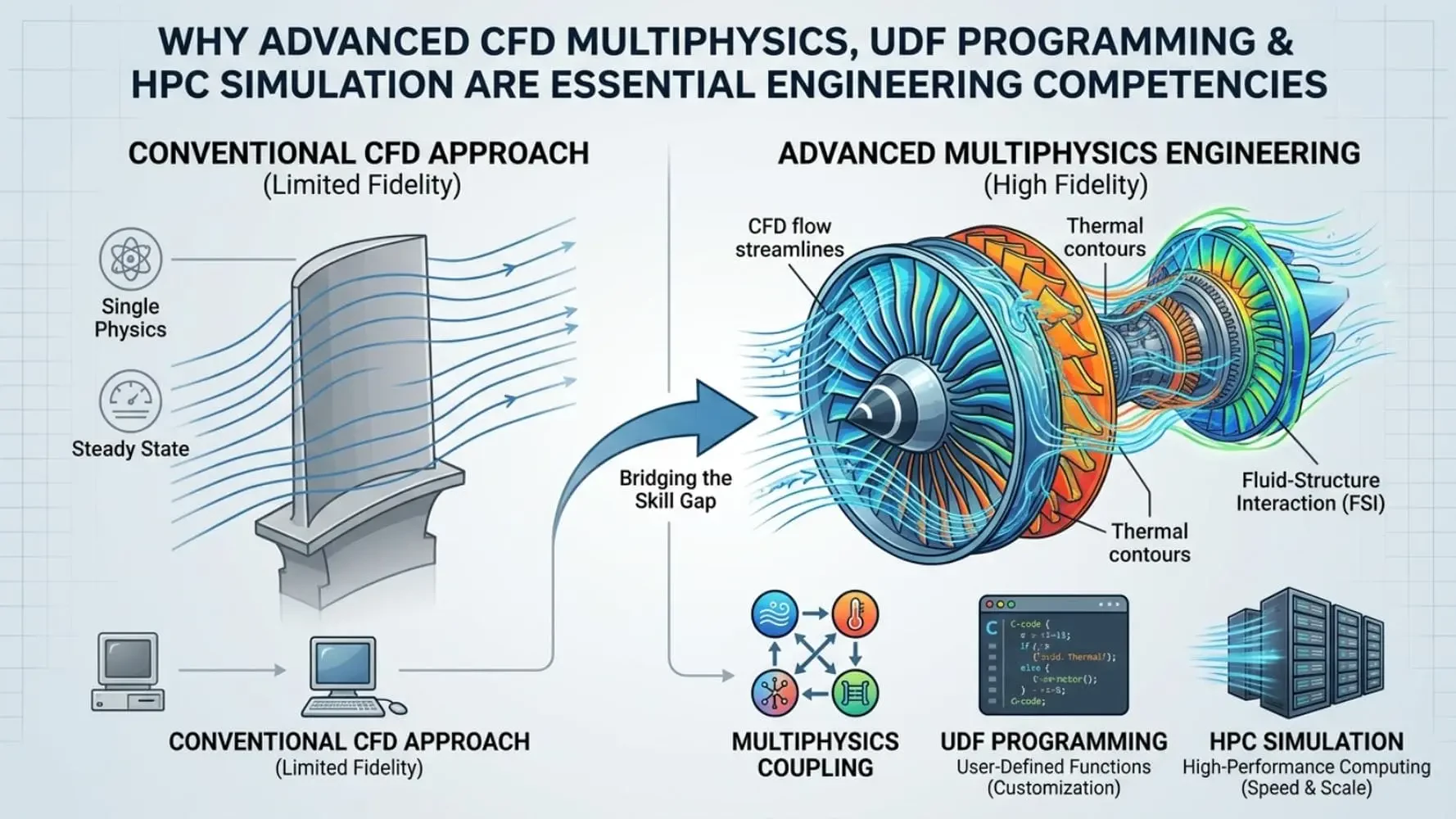
The industrial demand for engineers capable of advanced ANSYS Fluent simulation has grown substantially as simulation-driven design replaces physical prototyping. The bottleneck is not software access — it is the absence of engineers who understand model validity boundaries, can write UDFs that extend solver behavior, and can build a converging case from an undefined problem statement. This course addresses that gap directly, with industrial-grade projects built around real engineering decision points.
Technical CFD Competencies & ANSYS Fluent Solver Skills You Will Master in this Advanced CFD Course
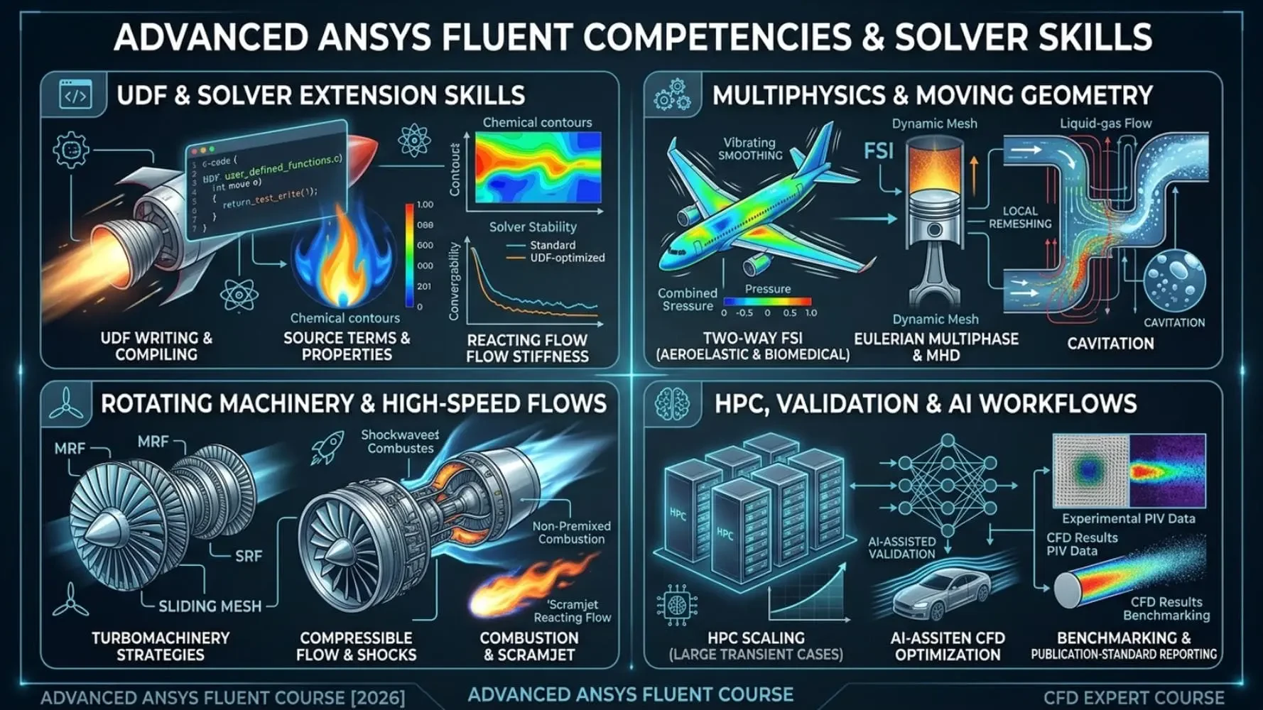
UDF & Solver Extension Skills
Writing, compiling, and hooking User-Defined Functions for source terms, boundary profiles, and material properties
Managing turbulence-chemistry interaction, solver stiffness, and convergence in reacting flow simulations
Multiphysics & Moving Geometry
Two-way fluid-structure interaction (FSI) for aeroelastic and biomedical applications
Dynamic mesh with spring smoothing, local remeshing, and RBF morphing
Eulerian multiphase modeling, MHD/EHD, cavitation, and PCM phase change
Rotating Machinery & High-Speed Flows
Selecting and validating MRF, SRF, and Sliding Mesh strategies for turbomachinery
Compressible flow with shocks, non-premixed combustion, and scramjet reacting flow
HPC, Validation & AI Workflows
Parallel partitioning and HPC scaling for large transient and multiphase cases
AI-assisted CFD for setup validation, post-processing, and parametric exploration
Result benchmarking against experimental data and publication-standard reporting
Expert CFD Course Modules: UDF, FSI, Combustion, Rotating Machinery, Multiphase & HPC Projects
ANSYS Fluent UDF Programming: Custom Source Terms, Boundary Profiles & Pulsatile Flow Simulation
This module transforms Fluent from a fixed-function tool into a programmable CFD simulation environment. Students write UDFs using DEFINE_SOURCE, DEFINE_PROFILE, and DEFINE_PROPERTY macros — applied to the Prandtl-number macro for temperature-dependent conductivity, pulsatile arterial flow velocity profiles for cardiovascular simulation, and tanker-truck sloshing with custom free-surface forcing. This capability is directly applicable in pharmaceutical mixing, biomedical device design, and industrial fluid systems where standard boundary options are physically insufficient.
Two-Way FSI & Dynamic Mesh CFD: NACA 0014 Aeroelasticity, Aortic Valve Displacement & Pipeline Pigging
Students implement two-way FSI on the NACA 0014 airfoil for aeroelastic flutter and on an aortic valve for leaflet displacement under physiological pressure. Dynamic mesh projects include pipeline pigging, golf-ball impact aerodynamics, and sea-robot locomotion — each requiring a different combination of spring smoothing, remeshing, and RBF morphing. Applications span wind turbine blade aeroelasticity, cardiovascular implant design, and subsea robotics.
Rotating Machinery CFD Simulation: MRF, SRF & Sliding Mesh for Compressors, Axial Fans & Twin-Screw Pumps
Students apply MRF, SRF, and Sliding Mesh methods to centrifugal compressor, multistage compressor, axial fan stage, and twin-screw pump configurations. The module teaches not just how to apply each method but when each is physically valid and where it introduces systematic error — the distinction that defines expert-level rotating machinery CFD for power generation, HVAC, aerospace propulsion, and industrial pump design.
Compressible Flow, Shock Simulation & Reacting Flow Combustion: Supersonic Nozzle, Steam Ejector & Scramjet CFD
Compressible flow projects cover supersonic nozzle separation and steam ejector simulation, where shock-boundary layer interaction and real-gas effects require precise boundary specification. Combustion projects span non-premixed combustion, species transport with finite-rate chemistry, and hypersonic scramjet combustion — managing turbulence-chemistry interaction, chemical stiffness, and coupled shock-reaction zone dynamics for aerospace propulsion and gas turbine combustor design.
Advanced Multiphysics CFD: MHD, FW-H Acoustics, Cavitation, PCM Solidification & Eulerian Multiphase in Fluent
This module covers the physics packages that separate an expert from an advanced user. MHD/EHD simulation targets electromagnetic pump design and plasma-assisted flow control. FW-H acoustics predicts aeroacoustic noise from rotating components for wind turbine and automotive compliance. Cavitation and phase-change mass transfer address hydraulic machinery erosion and refrigerant two-phase flow. PCM solidification/melting applies to thermal energy storage, and the Eulerian multiphase model handles boiling heat transfer in nuclear thermal-hydraulics and chemical reactor design.
HPC Parallel Computing & AI-Augmented CFD: Partitioning, Scaling & Parametric Exploration in ANSYS Fluent
This module covers parallel partitioning strategies, HPC scaling behavior analysis, and deployment on MR CFD’s dedicated ANSYS HPC infrastructure. The AI component addresses automated setup validation, pattern recognition in large post-processing datasets, and surrogate-based parametric CFD exploration — while establishing clear boundaries where physical judgment cannot be delegated to automated tools.
Industry-Standard CFD Engineering Skills & Simulation Workflows Developed in This Expert Course
Skill Category | Competencies Gained |
|---|---|
UDF & Solver Skills | UDF writing/hooking, stiff chemistry convergence, transient time-stepping |
Multiphysics Modeling | Two-way FSI, Eulerian multiphase, MHD/EHD, FW-H acoustics, cavitation, PCM |
Rotating Machinery CFD | MRF/SRF/Sliding Mesh selection, compressor & pump internal flow |
High-Speed & Reacting Flows | Shock-capturing, non-premixed combustion, scramjet species transport |
HPC & AI Workflows | Parallel scaling, AI-assisted post-processing, experimental benchmarking |
Real-World Industrial Applications of This ANSYS Fluent Expert Course
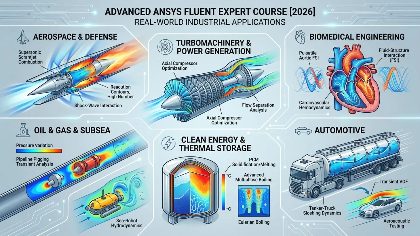
Aerospace & Defense: Supersonic nozzle aerodynamics, scramjet combustion, NACA aeroelastic flutter, FW-H aeroacoustic noise prediction
Turbomachinery & Power Generation: Centrifugal and multistage compressor optimization, axial fan aerodynamics, twin-screw pump design
Biomedical Engineering: Pulsatile arterial flow UDF simulation, aortic valve FSI, cardiovascular implant hemodynamics
Oil & Gas & Subsea: Pipeline pigging transient analysis, cavitation in hydraulic machinery, sea-robot hydrodynamics
Clean Energy & Thermal Storage: PCM solidification/melting, Eulerian boiling for nuclear thermal-hydraulics
Automotive: Tanker-truck sloshing dynamics, aeroacoustic compliance testing
Who Should Enroll in This Advanced ANSYS Fluent Expert CFD Course
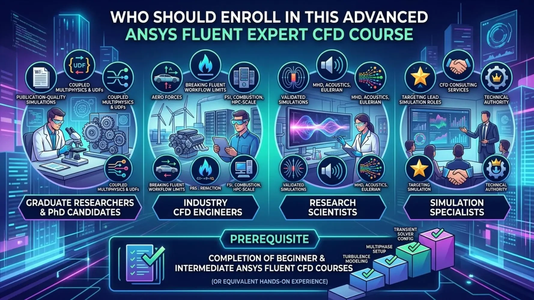
Graduate Researchers & PhD Candidates: Requiring publication-quality coupled multiphysics and UDF-driven simulations
Industry CFD Engineers: Who have reached the limits of standard Fluent workflows and need FSI, combustion, or HPC-scale multiphase capability
Research Scientists: Requiring validated MHD, acoustics, or Eulerian multiphase simulation for funded research projects
Simulation Specialists: Targeting lead simulation roles or ANSYS Fluent consulting services requiring expert-level technical authority
Prerequisite: Completion of the Beginner ANSYS Fluent CFD Course and the Intermediate ANSYS Fluent CFD Course, or equivalent hands-on experience in turbulence modeling, multiphase setup, and transient solver configuration.
Why MR CFD Delivers Unmatched Expert ANSYS Fluent & Advanced CFD Simulation Training
MR CFD is a specialized computational fluid dynamics training and consulting organization with a curriculum built from production consulting experience — not textbook exercises. Every project reflects real modeling decisions, convergence challenges, and validation benchmarks from industrial practice.
Production-Grade Projects: Every case presents a genuine engineering decision point
Industry-Standard Verification: Results benchmarked against experimental data and analytical solutions
Integrated HPC Infrastructure: Production-scale parallel simulation experience included
Internship-to-Consulting Pathway: Top graduates access MR CFD’s CFD internship program for live consulting project experience
ANSYS Fluent CFD Learning Path: Beginner Foundations to Expert Multiphysics Mastery
Level | Course | Core Focus |
|---|---|---|
Level 1 | Geometry, meshing, boundary conditions, steady-state setup | |
Level 2 | Turbulence modeling, multiphase, heat transfer, transient cases | |
Level 3 | This Course — Expert Complete CFD Course | UDFs, FSI, rotating machinery, combustion, HPC, AI workflows |
Enroll in the ANSYS Fluent Expert CFD Course & Achieve Simulation Mastery
Expert-level computational fluid dynamics demands more than software familiarity — it demands the engineering judgment to approach undefined coupled problems, select valid physical models, write the necessary UDFs, and deliver results that withstand rigorous technical scrutiny. This Advanced ANSYS Fluent CFD Course by MR CFD delivers that capability through production-grade projects and a structured three-course learning path.
Begin your enrollment through MR CFD’s CFD training courses and take the definitive final step toward Expert ANSYS Fluent simulation mastery.
You are ready if you can mesh confidently, set up both steady and transient cases, and read your own residuals without hand-holding. Comfort with turbulence modeling, multiphase, and heat transfer is assumed. If any of those still feel shaky, do Level Up to Intermediate first, because this course does not re-teach the interface.
Not strictly. This is the final stage of the three-course path, so it assumes everything the earlier two build toward, but you can start here if you already have equivalent hands-on experience with turbulence, multiphase, heat transfer, and transient setup. If you learned CFD on the job rather than in order, that counts.
Fluent is the main solver throughout, but the course also steps outside it on purpose: there is a plate heat exchanger built in ANSYS CFX and a silencer analysis in ANSYS Discovery. Seeing the same class of problem in a different solver helps you understand when to reach for which tool, which is part of thinking like an expert rather than a single-tool user.
ANSYS Fluent plus the geometry and meshing tools used across the lessons (Design Modeler, SpaceClaim, ANSYS Meshing, and Fluent Meshing), with a couple of lessons in ANSYS CFX and ANSYS Discovery. As with the earlier courses, you bring your own active ANSYS license, student or commercial.
The intermediate course gives you a second, harder project for every topic. This one takes the training wheels off entirely. Every project is chosen because it forces a modeling decision the interface cannot make for you: coupled physics, moving geometry, custom solver behavior through UDFs, and models large enough that hardware planning becomes part of the job.
That is the stated goal. By the end you should be able to take an undefined, coupled, real-world problem, pick the right models, apply the UDFs, build a case that actually converges, run it on HPC, and defend your results. That is the difference between someone who runs tutorials and someone a client can rely on.
No. Each project is self-contained, so you can go straight to the field, model, or module you need. Just keep in mind this is the expert tier, so if a project leans on something you skipped, the matching project in the earlier courses is the fastest way to fill the gap.