
Reach Professional-Grade ANSYS Fluent Training Course
Price:
$630
$39
Step up from expert to professional. This tier collects the most advanced project from every engineering field, flow model, and solver module in the MR CFD library — Over 40 specialized, multiphysics-heavy simulations that mirror the real consulting work CFD professionals get paid to deliver.
User-Defined Function: Property Macro UDF, Viscosity Relation
Property Macro: Temperature-Dependent Viscosity UDF in ANSYS FluentDescriptionWelcome to the tenth chapter of our comprehensive User-Defined Function (UDF) Training Course. This module focuses on using the Property Macro to model temperature-dependent fluid viscosity in CFD simulations with ANSYS Fluent.In this simulation, water flow through a pipe is modeled under varying temperature conditions that affect the fluid's viscosity. The project demonstrates the power of User-Defined Functions for creating realistic material property models that enhance flow simulations. The main components of the simulation include the 3D modeling of a pipe using Design Modeler, structured meshing with 134,400 cells using ANSYS Meshing, and a CFD simulation in ANSYS Fluent with a custom UDF implementation that defines the viscosity variation.MethodologyThis approach takes advantage of ANSYS Fluent's UDF capabilities to define a temperature-dependent viscosity model. The core of the simulation lies in the custom implementation of the viscosity variation through a User-Defined Function. The viscosity is defined as a custom function based on temperature ranges, implemented through the DEFINE_PROPERTY macro for advanced material property definition, and integrated into the flow simulation as a piecewise viscosity model.The User-Defined Function plays a crucial role in accurately representing the fluid's behavior under varying temperature conditions. The implementation follows a clear sequence: first, the custom temperature-dependent viscosity function is written; next, the DEFINE_PROPERTY macro is implemented; the UDF is then compiled and loaded into ANSYS Fluent; and finally, the fluid properties are set up to use the custom viscosity model.ResultsAfter running the simulation, a thorough analysis is carried out to evaluate how effectively the custom UDF models the temperature-dependent viscosity and influences the flow characteristics. The results include dynamic viscosity contours on various cross-sectional planes, temperature–viscosity correlation plots, and a comparison of the flow patterns with and without the temperature-dependent viscosity.This simulation highlights the importance of accurate material property models in CFD, with applications ranging from industrial process engineering to thermal management systems. The benefits of custom viscosity models include improved accuracy in predicting flow behavior under varying temperature conditions, greater simulation fidelity for heat transfer problems, and the ability to model complex non-Newtonian fluids and their temperature dependence.The techniques covered in this module open up many possibilities for advanced CFD research and industrial applications, such as integrating pressure-dependent viscosity models, developing multi-variable property functions for complex fluids, and applying these methods to multiphase flows with varying material properties. By mastering the Property Macro and UDF implementation in ANSYS Fluent, you will be equipped to tackle complex fluid dynamics problems with a high degree of control over material properties—knowledge that is invaluable for simulating and optimizing systems involving temperature-sensitive fluids across many engineering disciplines, from chemical processing to HVAC system design.
Reach Professional-Grade ANSYS Fluent Training Course
Price:
$630
$39
Step up from expert to professional. This tier collects the most advanced project from every engineering field, flow model, and solver module in the MR CFD library — Over 40 specialized, multiphysics-heavy simulations that mirror the real consulting work CFD professionals get paid to deliver.
-
Section 1
Engineering Fields
$18-
Slot Effect on Wing Aerodynamic Performance — ANSYS Fluent CFD SimulationA slot is a deliberate gap built into a wing that splits the airfoil into two sections, allowing high-pressure air from below to feed energy into the flow over the upper surface. It's a classic aerodynamic device used to delay separation and boost lift — the same principle behind the leading-edge slots and slats on many aircraft wings. This project simulates the steady airflow over a slotted NACA 4421 airfoil in ANSYS Fluent to quantify exactly how that slot changes the wing's lift and drag.The geometry is built in two dimensions in Design Modeler, with the slot placed near the leading edge so the airfoil is divided into two distinct elements. The domain is meshed in ANSYS Meshing, producing a grid of roughly 260,000 cells resolved around the airfoil surface and through the slot region.The simulation runs as a steady, incompressible case. Air enters the domain at 10 m/s and the airfoil is held at a zero-degree angle of attack, isolating the effect of the slot itself from any change in incidence. Turbulence is handled with the standard k-ε model, and the solver is run to convergence to extract the aerodynamic force coefficients.At the end of the solution, you generate 2-D contours of pressure, velocity, and turbulent (eddy) viscosity. The pressure field clearly shows the stagnation point at the leading edge, where pressure rises sharply as the flow is brought to rest. The computed force coefficients for the slotted airfoil are a drag coefficient of 0.0755 and a lift coefficient of 0.3764. Compared with a plain NACA 4421 at the same zero angle of attack — reported at roughly Cd = 0.06 and Cl = 0.1 — both coefficients rise with the slot present. The lift gain is substantial, confirming the slot's intended job, while the modest drag increase shows the trade-off that comes with it. By the end of this project, you'll be able to set up a multi-element airfoil simulation, choose appropriate turbulence and solver settings, and extract and interpret lift and drag coefficients to evaluate an aerodynamic modification.
Lesson 1 11m 3s -
Hydraulic Jump of Water in a Rectangular Channel — ANSYS Fluent CFD SimulationA hydraulic jump is what happens when fast, shallow water abruptly slows down: the flow height rises sharply, velocity drops, and energy is dissipated in a turbulent transition. It's a key phenomenon in open-channel and agricultural water systems — spillways, irrigation canals, and energy-dissipation structures all rely on understanding where and how strongly a jump forms. This project uses ANSYS Fluent to capture that transition and locate exactly where the jump occurs for two different inlet flow rates.The water–air system is modeled with the VOF (Volume of Fluid) multiphase approach, which tracks the free surface between the flowing water and the surrounding ambient air. The fluid domain is built in Design Modeler, and a structured mesh of 231,646 elements is generated in ANSYS Meshing.The case is solved as a steady, pressure-based simulation with gravity included (−9.81 m/s² in the Y-direction). Turbulence is modeled with the standard k-ε model using standard wall treatment, and the VOF model runs with implicit volume-fraction formulation and implicit body forces over two Eulerian phases (air and water). Air enters through a pressure inlet at zero gauge pressure, while water enters through a mass flow inlet. The simulation is run for two inlet water flow rates to compare their effect on the jump. Pressure–velocity coupling uses the SIMPLE scheme, with PRESTO! for pressure, second-order upwind for momentum, and Modified HRIC for the volume fraction.The results show the hydraulic jump forming at different downstream locations depending on flow rate: the jump occurs about 0.9 m downstream for the lower flow rate and about 2.8 m downstream for the higher one — the stronger flow carries its momentum farther before transitioning. By the end of this project, you'll be able to set up a free-surface VOF simulation, configure the appropriate solver and discretization schemes for two-phase open-channel flow, and predict where a hydraulic jump forms as a function of inlet conditions.
Lesson 2 26m 45s -
Octagonal Windcatcher Natural Ventilation — ANSYS Fluent CFD SimulationA windcatcher is a tall rooftop tower used for passive, energy-free ventilation — a centuries-old design still relevant in sustainable architecture. It captures ambient wind at roof level and channels it down into the building below, flushing out warm, stale indoor air and replacing it with fresh outside air. Internal walls and channels trap the incoming flow and guide it downward from the upper intake panels into the occupied space. This project uses ANSYS Fluent to simulate the airflow through an octagonal windcatcher and confirm that it ventilates the room beneath as intended.The windcatcher is placed inside a large open-domain environment with a horizontal wind of 10 m/s at atmospheric pressure. The geometry is built in Design Modeler and meshed in ANSYS Meshing with an unstructured grid of about 2.33 million cells.This is a fluid-only analysis with no heat transfer — the focus is purely on how the tower's geometry drives air movement. The key feature is the internal layout above the windcatcher: barrier surfaces are arranged so that some upper inlets face the wind directly while others are shielded from it. This sets up a pressure difference across the tower — the windward openings push air in, while the leeward openings generate suction — and that differential is what drives circulation down through the windcatcher shaft and into the room below.At the end of the solution, you generate velocity and pressure contours, along with velocity vectors and path lines. The windward side shows higher pressure than the leeward side, exactly as the design relies on. The flow visualizations confirm the intended behavior: air enters through the top panels, is guided and trapped by the interior walls, then descends and discharges through the lower panels into the interior space — showing the windcatcher works as designed. By the end of this project, you'll be able to set up an external-flow ventilation simulation in a large open domain, use barrier surfaces to create a driving pressure differential, and interpret pressure and flow fields to verify that a passive ventilation system performs as intended.
Lesson 3 16m 5s -
DescriptionThis project uses ANSYS Fluent to simulate how coronavirus-laden droplets released during speech can travel at sub–social-distance separations. We conduct and analyze the CFD study to assess transmission risk while talking.The scenario models exhaled particles from an infected speaker and their transport toward another person within a defined indoor volume. Geometry is built in DesignModeler as a 3D domain measuring 1.6 m × 2 m × 2.6 m, with two individuals facing each other 0.8 m apart. The infected person’s mouth serves as the particle source.Meshing is performed in ANSYS Meshing, producing 724,076 elements. Because dispersion evolves over time, a transient solver is employed.Talking MethodologyTo capture particle transport and deposition, the discrete phase model (DPM) is used, treating droplets as a dispersed phase moving through a continuous air field. Unsteady particle tracking is enabled with a 0.001 s time step.An injection is defined at the mouth surface with inert particles of 1×10⁻⁶ m diameter and 310 K temperature, released from 0 to 20 s. A custom profile prescribes the particle velocity and mass flow rate during speech, with a sinusoidal velocity history peaking at 0.33 m/s and the mass flow rate tied proportionally to that velocity. Turbulence is modeled with RNG k–ε, and the energy equation is solved to capture temperature effects.Talking ConclusionPost-processing provides particle tracks at multiple times, reported by residence time and instantaneous velocity. The results show particle emission occurs during the first 20 s; during the subsequent 20 s, only previously emitted particles continue to move within the gap between the individuals. Overall, the simulation indicates that speaking for 20 s without a mask can lead to particles reaching the other person by about 40 s, potentially exposing them to the virus.
Lesson 4 15m 17s -
Plasma Gasification Reactor — ANSYS Fluent CFD SimulationPlasma gasification is a high-temperature waste-treatment process that converts organic material into synthetic gas (syngas). An electric arc generates plasma hot enough to ionize and break down the feedstock, leaving behind syngas and an inert solid residue. It's used to treat waste and to process biomass and heavy hydrocarbons such as coal and petroleum sands — turning low-value or hazardous material into usable fuel gas. This project uses ANSYS Fluent to simulate the airflow and heat distribution inside such a reactor, capturing how the hot inlet streams behave as they meet and rise toward the outlet.The reactor is modeled in two dimensions in Design Modeler as a symmetrical chamber with two inlets — one on each side — and a single outlet along the top edge. The domain is meshed in ANSYS Meshing with a structured grid of 8,711 elements.The simulation captures the thermal-flow behavior of the reactor. Hot gas enters through the two side inlets at 0.1 m/s and 2000 K, and leaves through the top outlet at atmospheric pressure. The reactor's side walls are held at a fixed temperature of 600 K, representing heat loss through the chamber boundary. Running the case to convergence resolves how the two opposing inlet streams interact and how heat is carried through the chamber.At the end of the solution, you generate 2-D contours of pressure, velocity, and temperature, along with path lines and velocity vectors. The pressure drops as the flow approaches the outlet. The maximum velocity appears at the center of the chamber, where the two inlet streams collide and merge, while the highest temperatures sit at the inlets, where the hot 2000 K gas enters before mixing and cooling toward the walls. By the end of this project, you'll be able to set up a thermal-flow simulation with multiple opposing inlets, apply fixed-temperature wall conditions, and interpret how colliding streams shape the velocity and temperature fields inside a reactor.
Lesson 5 10m 39s -
Flat Plate Solar Collector — Conjugate Heat Transfer (CHT) ANSYS Fluent CFD SimulationFlat plate solar collectors (FPSC), and the photovoltaic-thermal (PV/T) systems built around them, convert sunlight into useful heat — typically by warming water that flows through pipes bonded to a sun-facing plate. How well they perform depends on the collector design, the materials in each layer, and where the collector sits and how it's tilted. This project uses ANSYS Fluent to model an FPSC installed in Doha at a 45° tilt, solving the full conjugate heat transfer (CHT) problem to see how solar radiation heats the water passing through the collector's pipes.The geometry is built in Design Modeler and meshed in ANSYS Meshing with a tetrahedral grid of roughly 5.59 million elements — a large mesh needed to resolve the thin solid layers, the pipe walls, and the water together as a coupled system.The simulation couples three physics together: the Navier–Stokes equations for the water flow, the energy equation for heat transfer through both fluid and solid, and the Discrete Ordinates (DO) radiation model for the incoming solar irradiation. Water enters at 300 K with a mass flow rate of 0.02 kg/s and exits at atmospheric pressure, while solar irradiation is set at 800 W/m². A key feature of the model is the heat generated inside the PV layer itself: rather than treating the panel as a simple absorber, the volumetric heat flux in the PV layer is computed from the solar flux, the glass transmittance, the PV absorption coefficient, the panel efficiency, and the PV layer thickness — then applied as a volumetric heat source. This is what makes the case a true PV/T simulation rather than a plain solar-heating one.At the end of the solution, the results show clearly how solar radiation raises the water temperature as it travels through the collector. The average water temperature reaches about 306.5 K, and the average PV layer temperature about 310.1 K — the panel running hotter than the water it's heating, as expected. By the end of this project, you'll be able to set up a coupled CHT simulation with radiation, apply the DO model for solar loading, implement a volumetric heat source from physical panel parameters, and interpret the temperature distribution across a multi-layer solar collector.
Lesson 6 20m 54s -
Server Room Cooling with 6 Cabinets — ANSYS Fluent CFD SimulationServer rooms generate large amounts of heat, and keeping that heat within a safe band is critical: manufacturers typically specify an operating range of about 10–32 °C, and drifting below or above that range creates unstable conditions that threaten the equipment. Cooling is therefore one of the core challenges in data-center design, alongside airflow planning, power redundancy, and fire suppression. This project uses ANSYS Fluent to model the airflow and temperature distribution inside a six-cabinet server room and determine whether the cooling keeps every rack within the safe thermal range.The room is modeled in three dimensions in Design Modeler, measuring 7 × 4 × 2 m, with six server cabinets each measuring 1 × 0.6 × 1.8 m arranged as heat sources. The domain is meshed in ANSYS Meshing with a structured grid of 448,000 elements.The simulation treats the room as a forced-convection problem. Cool air enters at 15 °C, and each of the six cabinet racks is modeled as a 400 W heat source. Because forced convection dominates over natural convection here, air density is taken as constant. The key variable studied is the inlet air speed, which is run at two values — 0.5 m/s and 1 m/s — to see how supply velocity affects how well the racks are cooled. The goal is to find conditions that hold the entire room within the safe sub-32 °C range.At the end of the solution, you generate 2-D and 3-D contours of temperature and streamlines, along with plots of the maximum and average fluid temperature. The results tell a clear engineering story: at the lower inlet speed of 0.5 m/s, the maximum temperature condition is not satisfied — parts of the room exceed the safe 32 °C limit. Raising the inlet speed to 1 m/s brings the maximum temperature down to around 30 °C, back inside the safe band. In other words, increasing the supply airflow directly improves rack cooling and resolves the overheating. By the end of this project, you'll be able to set up a 3-D forced-convection cooling simulation with multiple heat sources, run a comparative study across inlet conditions, and use temperature contours and bulk-temperature plots to verify that a cooling design meets a required thermal limit.
Lesson 7 11m 32s -
Tank Charge Between Two Reservoirs (Two-Phase) — ANSYS Fluent CFD SimulationThis project models the filling, or "charge," of a tank between two equal-height reservoirs using ANSYS Fluent. As water advances from one reservoir into the air-filled one, the two fluids exchange places — water flows in while air rises out — until the connected system settles into balance. A two-phase VOF approach captures the water–air interaction, reflecting the kind of phase separation and transfer operations that are common in chemical and petrochemical processing.The geometry consists of two 2-D reservoirs, each 1.25 × 2.5 m, built in Design Modeler and meshed in ANSYS Meshing with a structured grid of 32,510 cells.The simulation runs as a pressure-based, transient case with gravity enabled (−9.81 m/s² along Y). The water and air are tracked with the VOF model using two phases (air as primary, water as secondary), a sharp interface, and implicit formulation. Turbulence is handled with the realizable k-ε model and standard wall functions. Both the inlet and outlet vents are set to 0 Pa gauge pressure, so the flow is driven purely by gravity and the pressure imbalance between the reservoirs rather than by a forced inlet velocity — which is what makes this a natural transfer problem rather than a pumped one. Pressure–velocity coupling uses the Coupled scheme, with PRESTO! for pressure and a Compressive scheme for the volume fraction to keep the interface crisp. The case is initialized with the water region patched to a volume fraction of 1, then advanced with a 0.001 s time step over 10,000 steps.At the end of the solution, you generate 2-D contours of volume fraction, pressure, velocity, and turbulent kinetic energy, along with an animation of the transfer. The animation shows air rising as the water advances toward the air-filled tank. After several seconds, the system approaches hydrostatic balance — equal pressure at equal elevations across the two connected reservoirs — confirming the transfer reaches equilibrium as expected. By the end of this project, you'll be able to set up a transient gravity-driven VOF simulation, configure pressure-vent boundaries for a natural transfer process, patch initial phase distributions, and interpret how a two-phase system evolves toward hydrostatic equilibrium.
Lesson 8 23m 41s -
Towel Warmer Heat Transfer (Conjugate Heat Transfer) — ANSYS Fluent CFD SimulationA towel warmer is a heated rail mounted in a bathroom that warms and dries towels while adding gentle background heat to the room. Although it's an everyday appliance, simulating it well is a genuine multimode heat-transfer problem: heat conducts through the solid heating elements, drives buoyancy-driven natural convection in the surrounding air, and radiates to the nearby walls and towels — all three modes acting at once. This project uses ANSYS Fluent to model that coupled behavior, capturing how heat spreads from the warmer into the towels and the enclosed bathroom space, and where the design heats evenly versus where it leaves cold spots.The geometry is the towel warmer within its enclosed bathroom-like air domain, set up in Design Modeler and meshed in ANSYS Meshing, with the mesh resolving both the solid (heating element and structure) and the surrounding fluid region so the conjugate heat transfer can be captured across the solid–fluid interface.The simulation couples three heat-transfer mechanisms. Conduction is solved through the heating elements and warmer structure; natural convection is modeled as buoyancy-driven flow, where temperature differences set the air in motion and circulate heat around the warmer; and a radiation model accounts for radiative exchange between the warmer surface and the surrounding walls and towels — important in an enclosed space where radiation contributes meaningfully to the warming effect. Because the airflow is low-speed and buoyancy-driven, the turbulence treatment is chosen to suit natural convection rather than forced flow. The heating element is driven by a defined power or surface temperature, with ambient room conditions and material properties applied to the air and towels.At the end of the solution, you generate temperature contours across the warmer and the room, plus velocity vectors and pathlines that reveal the buoyancy-driven air-circulation pattern. From these you can assess how uniform the surface temperature is, estimate the heat-transfer rate from the warmer to the towels, and identify cold spots — regions of inefficient heating that point to design improvements. By the end of this project, you'll be able to set up a conjugate heat-transfer simulation that couples conduction, natural convection, and radiation in an enclosed space, select appropriate turbulence and radiation models for low-speed buoyancy-driven flow, and interpret the results to evaluate heating uniformity and energy efficiency in a household appliance.
Lesson 9 12m 54s -
Uniform Floor Heating System in a Closed Room CFD Simulation - HVAC: BEGINNER Delve into the intricate world of thermal dynamics with our comprehensive ANSYS Fluent tutorial on uniform floor heating in a sealed environment. This pivotal episode, part of our “HVAC: BEGINNER” course, showcases the power of Computational Fluid Dynamics (CFD) in analyzing and optimizing radiant heating solutions for controlled spaces. Ideal for aspiring HVAC engineers, building physics enthusiasts, and CFD learners, this hands-on tutorial guides you through the nuanced process of modeling and evaluating floor heating performance in a completely enclosed room. Gain invaluable insights into natural convection, thermal stratification, and the ideal gas model, all while mastering essential CFD simulation techniques using ANSYS Fluent. Understanding Floor Heating Dynamics in Sealed Environments Begin your exploration of this unique heating scenario with these fundamental concepts: Principles of Natural Convection in Enclosed Spaces Master the physics driving air movement in sealed, heated rooms: Understand the mechanism of buoyancy-driven flows in the presence of temperature gradients Learn about the formation and behavior of convection cells in enclosed environments Explore the impact of room geometry on natural convection patterns Ideal Gas Model and Its Relevance in HVAC Simulations Gain crucial insights into accurate air behavior modeling: Analyze the principles of the ideal gas law and its application in CFD simulations Understand the importance of density variations in natural convection scenarios Explore the limitations and advantages of using the ideal gas model for indoor air simulations Setting Up Your Closed Room Floor Heating CFD Simulation Dive into the intricacies of modeling this controlled heating scenario with ANSYS Fluent: Sealed Room Geometry and Mesh Generation Develop skills in preparing an accurate model for CFD analysis: Learn to create a simple, perfectly sealed rectangular room with a uniform floor heating element Understand the importance of mesh quality and refinement near the heated floor and room boundaries Explore best practices for representing adiabatic walls and ceilings in the CFD model Implementing Boundary Conditions and Material Properties Master the art of setting up a realistic simulation scenario: Learn to define appropriate thermal boundary conditions for the heated floor and insulated surfaces Understand how to implement the ideal gas model for air in ANSYS Fluent Develop skills in configuring radiation properties for surfaces to account for all heat transfer mechanisms Running Your Floor Heating Performance Simulation Experience the power of CFD in analyzing complex thermal environments: Solver Configuration for Natural Convection Flows Gain insights into the computational aspects of simulating buoyancy-driven flows: Understand the selection of appropriate turbulence models for enclosed natural convection Learn about transient simulation techniques for capturing the dynamics of room heating Explore convergence strategies for challenging, low-velocity thermal flow problems Advanced Post-Processing for Thermal Comfort Analysis Develop skills in extracting meaningful data from your simulation: Learn to create temperature contours and velocity vector fields to visualize thermal stratification and airflow patterns Understand how to generate streamlines to illustrate convection cell structures in the enclosed space Explore techniques for calculating and visualizing key performance indicators like heating uniformity and efficiency Analyzing Floor Heating System Performance Apply your CFD skills to evaluate the effectiveness of the floor heating in a sealed room: Temperature Distribution and Thermal Stratification Assessment Master techniques to analyze heating efficiency and comfort: Learn to interpret vertical temperature gradients and assess thermal stratification effects Understand how to evaluate the uniformity of heating across the room’s floor area Develop skills in quantifying the impact of room dimensions on overall heating performance Natural Convection Pattern and Heat Transfer Evaluation Gain insights into the complex air movement in sealed, heated spaces: Learn to analyze the formation and structure of convection cells within the room Understand how to evaluate heat transfer rates from the floor to the room air Explore methods for optimizing floor temperature to achieve desired comfort levels while minimizing energy use Optimizing Floor Heating Design for Sealed Environments Apply your newfound knowledge to enhance radiant heating system performance: Parametric Studies for Performance Enhancement Learn to conduct systematic analysis of floor heating configurations: Understand how to modify floor temperatures and assess their impact on heating dynamics Learn to evaluate the effects of room aspect ratios on natural convection patterns Develop skills in interpreting CFD results to make informed decisions on radiant heating design Innovative Strategies for Efficient Sealed Space Heating Explore the potential of advanced radiant heating approaches: Learn to assess the benefits of variable temperature floor heating for improved comfort Understand how to integrate CFD insights into smart heating control algorithms for sealed spaces Develop skills in proposing and validating energy-efficient heating strategies for controlled environments Why This Episode is Crucial for Future HVAC Innovators This “Uniform Floor Heating System in a Closed Room CFD Simulation” episode offers unique benefits for those aiming to excel in advanced HVAC design and analysis: Hands-on experience with industry-standard CFD software applied to a controlled radiant heating scenario In-depth understanding of natural convection phenomena and their impact on indoor thermal environments Insights into the application of the ideal gas model for accurate air behavior simulation in HVAC contexts Foundation for analyzing and optimizing heating systems in diverse sealed environments, from residential spaces to controlled industrial settings By completing this episode, you’ll: Gain confidence in setting up and running sophisticated CFD simulations for enclosed thermal environments in ANSYS Fluent Develop critical skills in interpreting complex temperature and airflow patterns in spaces with radiant floor heating Understand the fundamental principles of effective heating design for sealed rooms and controlled environments Be prepared to tackle more advanced HVAC challenges and contribute to innovative climate control solutions for specialized applications Embark on your journey towards mastering advanced HVAC technologies with this essential episode from our “HVAC: BEGINNER” course. Unlock the potential of CFD simulation in optimizing radiant heating systems, and transform your approach to creating energy-efficient, comfortable indoor environments in controlled spaces!
Lesson 10 17m 38s -
Flood Over a Bridge — ANSYS Fluent CFD SimulationA flood occurs when water overflows onto land that is normally dry — when a river exceeds its channel capacity, a levee is overtopped, or rainwater accumulates on saturated ground. Floods are a central concern in hydrology, civil engineering, and public health, and they pose a serious threat to man-made structures in a river's floodplain. This project uses ANSYS Fluent to simulate a flood surging through a dry riverbed and striking a bridge, with the goal of quantifying the forces the flood imposes on the bridge's pillars.The geometry is built in Design Modeler and meshed in ANSYS Meshing with an unstructured grid of 844,311 elements.The water–air system is modeled with the VOF (Volume of Fluid) multiphase approach, which tracks the free surface between the advancing flood water and the surrounding air. Water enters the computational domain — a dry river — at a velocity of 10 m/s, representing the incoming flood front. The simulation is run in transient, 3-D form with gravity enabled (−9.81 m/s² in the Y-direction), and turbulence is handled with the standard k-ε model. The transient setup is essential here: a flood is an inherently time-dependent event, and capturing how the water front advances and loads the structure over time is the whole point.At the end of the solution, the results show clearly how a flood can damage and ultimately destroy a man-made structure like a bridge. One of the most important factors is the shear stress exerted on the bridge's pillars, which the simulation shows to be considerable. This kind of result has direct engineering value: it can inform the design of bridge pillars capable of withstanding extreme events like floods — choosing pillar shapes and structures that reduce the hydrodynamic loading. By the end of this project, you'll be able to set up a transient 3-D free-surface VOF simulation, model a flood front advancing through a domain, and extract structural loads such as shear stress on submerged structures to support resilient civil engineering design.
Lesson 11 25m 29s -
This project simulates the motion of a jet ski at the interface between water and air, capturing how a floating body disturbs the free surface as it moves. Flow around floating objects — boats, ships, jet skis — is one of the most common two-fluid phenomena around us, and wherever two fluids meet, the interaction and deformation of the interface becomes the central engineering question. Here the goal is to see how the jet ski rides the surface and reshapes the water behind it.The physics is handled with the Volume of Fluid (VOF) multiphase model, which tracks the sharp water–air interface as it deforms around the moving body — the standard tool for free-surface and open-channel problems where the shape of the surface is itself a key result.Setup: the computational domain has an inlet where water enters at a mass flow rate of 50,000 kg/s and a pressure outlet, with the jet ski floating at the interface. Geometry is built in ANSYS Design Modeler and meshed in ANSYS Meshing as an unstructured mesh (~1,748,941 elements) — unstructured here to wrap cleanly around the curved hull geometry.What the results show: contours of pressure, velocity, velocity vectors, and water volume fraction. The volume-fraction field captures the free surface clearly and shows how the phases interact around the floating body — the jet ski is pushed by the flow, and a distinct wake sequence forms behind it, with water lifted above the undisturbed surface level. That surface jump is exactly the behavior you'd expect from a jet ski's interaction with the water, recovered directly from the simulation.You'll learn to: set up a VOF water–air free-surface case around a floating body, define mass-flow inflow and pressure-outlet conditions, and read free-surface deformation and wake structure from volume-fraction and velocity fields.
Lesson 12 22m 14s -
Jet Engine Intake (3-D Internal Aerodynamics) — ANSYS Fluent CFD SimulationThe intake is the first component of a jet engine, and its job is deceptively difficult: it has to deliver air to the engine face smoothly, with as little pressure loss and as much uniformity as possible, across a wide range of flight conditions. Poor intake performance — distorted or non-uniform flow reaching the compressor — directly degrades engine efficiency and can threaten stable operation. This project uses ANSYS Fluent to simulate the airflow through a jet engine intake, examining the pressure and velocity fields inside the duct and the uniformity of the flow arriving at the engine face.The simulation works from a 3-D intake geometry imported as a prepared mesh, so the focus stays on the flow physics and solver setup rather than geometry creation. Boundary conditions are configured to represent the operating conditions a jet engine intake experiences — an incoming air stream at the intake entrance and the engine face as the downstream boundary — and the case is run to convergence to resolve how the air accelerates, turns, and redistributes as it moves through the duct.At the end of the solution, you generate pressure and velocity contours through the intake, along with flow visualizations that reveal how the air interacts with the intake geometry. From these you can assess two things that matter most for intake performance: the pressure and velocity distribution along the duct, and the flow uniformity at the engine face — the degree to which the air arriving at the compressor is even rather than distorted. By the end of this project, you'll be able to set up and run a 3-D internal-aerodynamics simulation from an imported mesh, apply realistic intake boundary conditions, and post-process the results to evaluate pressure recovery and flow uniformity — the core metrics that drive intake design decisions in aerospace engineering.
Lesson 13 8m 27s -
Solar Water Heater with PCM Thermal Storage (Solidification & Melting) — ANSYS Fluent CFD SimulationPhase change materials (PCMs) store and release large amounts of energy as they melt and freeze over a nearly constant temperature range — the latent heat of the phase change. That makes them a powerful, self-regulating way to store thermal energy, and they've become especially popular for solar applications, where heat is available intermittently and needs to be banked for later. This project uses ANSYS Fluent to study a solar water heater that uses encapsulated PCM in its storage tank, modeling how the material melts and solidifies as it charges and discharges heat — a modern approach to improving solar thermal storage.The geometry, built in Design Modeler, is the annular chamber between two coaxial tubes, with the space between them filled with PCM. It's meshed in ANSYS Meshing with an unstructured grid of 5,803 cells. The PCM region's inner wall is held at a fixed temperature of 603.3 K with a thickness of 0.0015 m, driving heat into the material, while the outer wall is set adiabatic so the study isolates the PCM's thermal response.The simulation activates the energy equation to resolve the temperature field, and the core physics is handled by Fluent's Solidification and Melting model, which tracks the PCM changing phase between solid and liquid as the temperature varies inside the storage region. The Boussinesq model is used to capture the buoyancy effects from density changes with temperature — the natural convection that develops in the molten PCM and strongly influences how heat spreads. Setting up the phase-change model requires defining the solidus and liquidus temperatures and the latent heat of melting for the material. The project is framed to investigate several factors: the effect of the PCM's melting/freezing temperature, the effect of the PCM volume, and a comparison against a tank with no PCM at all.At the end of the solution, you generate contours of temperature, velocity, pressure, and liquid volume fraction. The results show full consistency between the temperature field and the liquid fraction: as the PCM heats up under the inner-wall boundary condition, it melts and the liquid fraction rises, and as it cools, the phase change reverses and the material solidifies. By the end of this project, you'll be able to set up a phase-change simulation using the Solidification and Melting model, apply the Boussinesq approximation for buoyancy-driven convection in a melting material, define the thermophysical parameters that govern phase change, and interpret coupled temperature and liquid-fraction results to evaluate a PCM-based thermal storage design.
Lesson 14 15m 34s -
Axial Flow Fan Stage (Rotor–Stator, MRF) — ANSYS Fluent CFD SimulationAn axial fan stage is a rotor–stator assembly that produces steady, directed airflow for industrial uses such as cooling freshly painted body parts. The two components share the work: the spinning rotor blades add energy to the air and induce swirl, and the stationary stator blades then straighten that swirling flow so it leaves the stage roughly normal to the outlet. This project uses ANSYS Fluent to model both the rotating and stationary zones of such a fan stage and evaluate its aerodynamic performance — a classic, transferable introduction to turbomachinery CFD.The 3-D rotor–stator geometry is built in Design Modeler with separate rotating and stationary zones defined, then meshed in ANSYS Meshing with about 244,675 cells. To keep the computation efficient, a periodic boundary condition is used to model only a single slice of the fan rather than the full annulus — the standard way to cut the cost of a turbomachinery analysis without losing fidelity.The rotation is handled with the Moving Reference Frame (MRF) method, which simulates the rotor spinning at 1800 rpm while the stator stays fixed — a steady-state approach to rotating machinery that avoids the expense of a fully transient moving mesh. Turbulence is modeled with the standard k-ε model across the rotating flow field.At the end of the solution, you generate 2-D and 3-D contours of pressure and velocity, along with streamlines and velocity vectors that clearly reveal the swirl induced by the rotor and its correction by the stator. From the results you extract the key turbomachinery performance metrics: a rotor tip linear velocity of about 31 m/s, a Tip Speed Ratio (TSR) of 4, and an outlet airflow rate of 16.14 L/s. By the end of this project, you'll be able to build a rotor–stator geometry with distinct motion zones, apply periodic boundaries to model a representative slice, set up the MRF method for rotating machinery, and post-process the flow to compute the performance metrics that define fan and compressor behavior — a workflow that transfers directly to blowers, axial compressors, pumps, and ventilation fans.
Lesson 15 14m 42s -
Profile Macro: Advanced UDF for Pressure Profiles in ANSYS FluentWelcome to the ninth chapter of our comprehensive User-Defined Function (UDF) Training Course. This module focuses on implementing the Profile Macro to create realistic pressure distributions in urban CFD simulations using ANSYS Fluent.Project Overview: Urban Area Air Pressure SimulationIn this advanced CFD simulation, we model air pressure distribution in a simplified urban environment, considering the natural pressure variation with altitude. This project demonstrates the power of User-Defined Functions in creating realistic boundary conditions for complex environmental simulations.Key Simulation Components3D geometry modeling of urban area using Design ModelerStructured meshing with 118,400 cells via ANSYS MeshingCFD simulation using ANSYS Fluent with custom UDF implementation for pressure profileMethodology: Implementing Profile Macro in UDFOur approach leverages ANSYS Fluent’s UDF capabilities to define a height-dependent pressure profile at the inlet boundary. The core of this simulation lies in the custom implementation of atmospheric pressure variation using a User-Defined Function.Pressure Profile Modeling TechniquesCustom pressure function based on height (Y-coordinate)Implementation of DEFINE_PROFILE macro for advanced boundary condition definitionIntegration of atmospheric pressure model into urban flow simulationUDF Implementation and Simulation ProcessThe User-Defined Function plays a crucial role in setting up realistic inlet conditions for the urban airflow simulation. We’ll guide you through the process of writing and integrating the UDF into your ANSYS Fluent simulation.Step-by-Step UDF IntegrationWriting the custom pressure profile functionImplementing the DEFINE_PROFILE macroCompiling and loading the UDF into ANSYS FluentSetting up the inlet boundary condition with the custom pressure profileResults Analysis and VisualizationAfter running the simulations, we conduct a thorough analysis to evaluate the effectiveness of our custom UDF in creating realistic pressure distributions within the urban environment.Performance Metrics and VisualizationPressure contours at inlet boundary and cross-sectional planesVertical pressure profile plots at inlet and central domain locationsComparison of UDF-generated profiles with theoretical atmospheric modelsAdvanced Insights: Enhancing Urban Flow SimulationsThis simulation provides valuable insights into the importance of accurate pressure profiles in urban CFD simulations, with applications ranging from city planning to pollution dispersion studies.Applications and Benefits of Custom Pressure ProfilesEnhanced accuracy in predicting urban airflow patternsImproved simulation fidelity for tall building aerodynamicsAbility to model complex atmospheric conditions in urban environmentsFuture Directions and Research OpportunitiesThe techniques learned in this module open up numerous possibilities for advanced CFD research and urban planning applications. Consider exploring:Integration of temperature and density variations in atmospheric profilesDevelopment of time-dependent atmospheric boundary conditionsApplication to large-scale urban heat island effect studiesBy mastering the Profile Macro and UDF implementation in ANSYS Fluent, you’re equipped to tackle complex environmental flow problems with unprecedented control over boundary conditions. This knowledge is invaluable for CFD professionals looking to simulate and optimize urban environments, assess building ventilation, or study pollutant dispersion in cities.
Lesson 16 17m 24s
-
-
Section 2
Flow Models
$9-
Vortex Flame Combustion Chamber, 4-Inlet (Methane and Air) — ANSYS Fluent CFD Simulation TrainingThis project simulates the vortex flame inside a combustion chamber using ANSYS Fluent, with the full case analyzed through CFD post-processing.The geometry is a three-dimensional cylindrical combustion chamber built in Design Modeler. Air enters through four inlet sections arranged radially around the chamber, while fuel enters through four inlet sections positioned axially at the top. A single outlet at the bottom of the chamber discharges the combustion products.The mesh was generated in ANSYS Meshing using a structured grid, with a total of 725,521 elements.MethodologyThe chamber has a cylindrical structure in which the reactants — fuel and air — enter separately through four inlets in the upper region, and the reaction products exit from the bottom.Air enters radially through four inlets spaced 90 degrees apart around the outer circumference of the chamber, while methane is injected directly into the chamber interior through the remaining four inlets. This arrangement establishes the swirling, vortex-shaped flame at the heart of the model.The chemical reaction between air and methane is modeled with the Species Transport model, involving five species: O₂, N₂, CH₄, CO₂, and H₂O. The incoming air contains a mass fraction of 0.23 oxygen, with a flow rate of 0.001135845 kg/s at 300 K. The fuel enters simultaneously at a flow rate of 0.0000645 kg/s, also at 300 K.The outer wall is treated as a convective boundary exchanging heat with the surroundings, with an ambient (free-stream) temperature of 300 K and a heat transfer coefficient of 25 W/m²·K.The RNG k-epsilon turbulence model and the energy equation are both activated to resolve the turbulent flow field and compute the temperature distribution throughout the domain.ResultsThe solution yields 2D and 3D contours of pressure, temperature, velocity, and the mass fractions of O₂, CH₄, H₂O, CO₂, and N₂.The contours show that as combustion takes place between fuel and air, temperature rises sharply near the chamber inlets. As the reaction proceeds, the methane mass fraction decreases while the mass fractions of the combustion products — CO₂ and H₂O — increase accordingly.
Lesson 1 15m 54s -
Wind Tunnel Drag Analysis — ANSYS Fluent CFD Simulation TrainingThis project models a wind tunnel and a specific body placed inside it using ANSYS Fluent, with the goal of investigating the drag force acting on the body.The geometry was created in ANSYS Design Modeler® and meshed in ANSYS Meshing® using an unstructured grid, for a total of 179,542 elements.BackgroundThe wind tunnel is one of the most widely used aerodynamic testing tools in use today. Among the many experiments it enables are tests of various structures, including airfoils, aircraft, and static bodies. These experiments are typically aimed at studying aerodynamic behavior and visualizing the flow lines around the test object.Wind tunnels can also be used for free-fall tests, examining how airflow affects a falling object. Because forces such as drag have a significant influence on a body's behavior, quantifying them is essential — and CFD provides an effective means of doing so.MethodologyA density-based (compressible flow) solver is used in this simulation, and the energy equation is activated accordingly to capture the compressible-flow physics.ResultsThe solution produces contours of velocity, pressure, temperature, and related quantities for a range of inlet Mach numbers. The velocity vectors reveal the formation of separation vortices behind the body. As a result of this separation, the flow turbulence in the wake is substantial — noticeably greater than in the rest of the computational domain.
Lesson 2 14m 42s -
Lifting Dam (Dam Break) — ANSYS Fluent CFD Simulation TrainingThis project presents a numerical simulation of a lifting dam (dam break) using ANSYS Fluent. The VOF (Volume of Fluid) model is used to capture the two fluid phases, with the goal of studying how the free surface of the fluid evolves over time. Two cases are examined: in the first, the flow continues freely after the dam is lifted, while in the second, it encounters an obstacle in its path.Geometry & MeshThe two-dimensional geometry was created in SpaceClaim, with a computational domain measuring 70 mm in length and 40 mm in height.Meshing was performed in ANSYS Meshing using an unstructured grid throughout. Case 1 contains 86,611 elements, while Case 2 contains 132,614 elements.MethodologySeveral assumptions underpin the model. Because the flow is incompressible, a pressure-based solver is selected, and the simulation is run as transient. Gravity is applied at −9.81 m/s² along the Y-axis. The two phases — air (density 1.225 kg/m³, viscosity 1.7894e-05 kg/m·s) and liquid water (density 998.2 kg/m³, viscosity 0.001003 kg/m·s) — are modeled with the Volume of Fluid approach using an explicit, sharp-interface formulation and implicit body forces.The laminar viscous model is used to solve the flow-field equations, with the SIMPLE scheme for pressure–velocity coupling. Momentum is discretized using second-order upwind, while pressure uses the PRESTO! scheme. The solution is initialized with the standard method, after which the water phase is patched into the initial region (volume fraction = 1). The calculation runs with adaptive time advancement over 2000 time steps at a step size of 0.0005 s.ResultsThe simulation tracks the free surface of the fluid as the dam is lifted. Once the solution is complete, contours of velocity, pressure, and volume fraction are extracted. In the second case, after the flow strikes the barrier it rises to a relatively high level, driven by the high kinetic energy present in the initial moments of the flow.
Lesson 3 17m 36s -
Particle-Laden Flow in a Micro-Bearing (DPM) — ANSYS Fluent CFD Simulation TrainingDescriptionIn certain industries — such as Microelectromechanical Systems (MEMS) and microfiltration — micro-channels and micro-bearings with flow thicknesses on the micrometer scale can carry particles on the nanometer scale. Under these conditions, the effect of the carried particles on the frictional force acting on the channel or bearing wall becomes very important. This project uses ANSYS Fluent and the Discrete Phase Model (DPM) to investigate how this wall frictional force differs with and without the presence of particles. The particles are spherical anthracite grains 400 nm in diameter, and the two-way interaction between the particles and the fluid is taken into account.The geometry consists of two concentric cylinders with diameters of 100 and 70 micrometers, drawn in ANSYS SpaceClaim. The outer cylinder rotates while the inner cylinder remains stationary. The mesh was generated in ANSYS Meshing and comprises 51,840 hexahedral elements — a density that resolves the flow dynamics, turbulence effects, and particle distribution within the domain. The element size is kept larger than the particle size to ensure proper particle tracking.MethodologyA pressure-based, transient solver is used to track the particle injection over time and capture the interaction between the particles and the fluid. The fluid filling the gap between the cylinders is Polyalphaolefin (PAO) 68. The SST k-omega turbulence model is adopted for its effectiveness in capturing the complex flow that develops around the rotating cylinder, and a suitable wall function resolves the near-wall region — essential for accurately representing the fluid–particle interactions near the walls and the resulting frictional force. Appropriate particle-dynamics forces and models are also included to improve the accuracy of the DPM settings.Results & ConclusionThe simulation yields the following results:The frictional force on the inner cylinder wall increases over time, while the frictional force on the outer cylinder wall decreases over time.In both the with-particle and without-particle cases, the frictional force on the outer cylinder wall exceeds that on the inner cylinder wall. This is likely because the outer cylinder is the rotating one, and the frictional force is proportional to the velocity gradient.The wall frictional force is higher when particles are present, because the particles raise the effective viscosity of the medium and thereby increase the friction.The plots show that, for the inner cylinder, the problem reaches steady state after 27 ms without particles and after 34 ms with particles. For the outer cylinder, steady state is reached after 11 ms without particles and after 20 ms with particles. Overall, then, the case without particles reaches steady state after 27 ms, while the case with particles reaches steady state after 34 ms.
Lesson 4 14m 30s -
Non-Newtonian Blood Pulsatile Flow in a Vein — ANSYS Fluent CFD Simulation TrainingThis project simulates non-Newtonian, pulsatile blood flow through a vein using ANSYS Fluent, with the full case analyzed through CFD post-processing.The working fluid is blood, a non-Newtonian fluid. Non-Newtonian fluids are those whose viscosity changes with shear rate, meaning they have no single fixed viscosity. In such fluids the relationship between shear stress and applied strain rate is nonlinear, so no constant viscosity coefficient applies. The simulation is run as transient over 0.5 s, and a User-Defined Function (UDF) is applied to model the pulsing of the blood flow. Because blood flow is not steady but pulsed, the velocity is prescribed as a periodic function through the UDF code.The geometry was created in Gambit. The model consists of a main cylindrical vessel and two smaller branch vessels of reduced size and diameter — one branching at a 90-degree angle and the other with a 45-degree curvature. It has one inlet section and two outlet sections.Meshing was performed in ANSYS Meshing using an unstructured grid, for a total of 397,388 cells.MethodologyThe working fluid is blood, with a density of 1050 kg/m³. Because blood is non-Newtonian, its viscosity is described using the Carreau model with appropriate parameters.Newtonian fluids maintain a constant viscosity under applied force, whereas non-Newtonian fluids exhibit variable viscosity, of which there are several types. Time-dependent non-Newtonian fluids fall into two categories: rheopectic fluids, such as printer ink and cream, whose viscosity increases over time under load, and thixotropic fluids, such as honey, whose viscosity decreases as force is applied. Time-independent non-Newtonian fluids divide into three groups: dilatants, such as starch and clay, whose viscosity depends only on the magnitude of the applied force; pseudoplastics, such as greases, paints, soaps, and ketchup, whose viscosity is inversely related to the applied force; and Bingham fluids, such as toothpaste and silica nanocomposites, which require a threshold stress before they begin to flow.In this simulation, blood is treated as a pseudoplastic non-Newtonian fluid defined by the Carreau model. This model spans a wide range of fluid behavior by fitting a curve that matches both Newtonian and shear-thinning (pseudoplastic) responses.ResultsAfter the solution is complete, contours of pressure and wall shear stress are obtained at several time instants. The results confirm that the flow inside the vessel is fully pulsatile, since the pressure varies over time. They also show that pressure and wall shear stress are correlated: as the pressure inside the vessel rises, the wall shear stress increases accordingly.
Lesson 5 24m 52s -
Wide-Edge (Broad-Crested) Spillway — ANSYS Fluent CFD Simulation TrainingIntroductionA wide-edge (broad-crested) spillway is a cascading structure with a long horizontal crown aligned with the flow direction, such that the error arising from the hydrostatic pressure distribution can be neglected thanks to the acceleration of the radial flow. These spillways operate so that the upstream flow is subcritical while the flow over the spillway itself becomes supercritical, creating a flow-control section above the crown. One characteristic of these structures is that, a short distance from the crown, the flow lines run nearly parallel.In this type of spillway, the crest is wide and substantial relative to the other dimensions. The crowns may be wide, horizontal, or follow a specific curvature. Although they can be used to measure discharge, they serve most often as dam spillways — and sometimes as the dam itself, when water is allowed to pass through — and can store large volumes of water when needed.Project DescriptionThis project investigates the flow inside a wide-edge spillway using ANSYS Fluent. There is a deliberate elevation difference between the main channel and the sub-channel, in part to store a portion of the flowing water. The RNG k-epsilon model solves the turbulent flow equations, while the multiphase VOF model captures the two phases of water and air within the open channel. Water enters the channel at a mass flow rate of 65 kg/s and passes into the second channel after striking the middle section of the spillway.Geometry & MeshThe geometry was created in ANSYS Design Modeler and meshed in ANSYS Meshing using a structured grid, for a total of 981,900 elements.MethodologySeveral key assumptions underpin the model. The simulation uses a pressure-based solver and is run as steady-state, so the results do not vary with time. Gravity is applied at −9.81 m/s² in the Y direction.Turbulence is modeled with the RNG k-epsilon model using standard wall functions, and the two phases — air as the primary phase and water as the secondary phase — are handled with the VOF approach. Water enters through a mass-flow inlet (65 kg/s) defined as an open-channel boundary, with a free-surface level of 0.08 m, a bottom level of 0 m, and density interpolation taken from the neighboring cell. The outlets are set as pressure outlets, and the walls are treated as stationary.For the solution methods, pressure–velocity coupling uses the SIMPLE scheme. Pressure is discretized with PRESTO! and momentum with second-order upwind, while volume fraction, turbulent kinetic energy, and turbulent dissipation rate all use first-order upwind. The solution is initialized with the standard method: gauge pressure 0 Pa, velocity 0 m/s, turbulent kinetic energy 1 m²/s², turbulent dissipation rate 1 m²/s³, and water volume fraction 0.ResultsThe water volume fraction contour shows that, because of the height difference and the absence of any inlet flow in the sub-channel, the water volume fraction takes nonzero values in the upper part of the sub-channel. Once the solution is complete, 3D contours of pressure, velocity, volume fractions, and related quantities are extracted and presented.
Lesson 6 22m 21s -
Steam Methane Reforming (SMR) Reactor — ANSYS Fluent CFD Simulation TrainingWhat You'll BuildThis lesson walks you through a CFD simulation of Steam Methane Reforming (SMR), the most widely used industrial route for producing hydrogen from hydrocarbon fuels. In an SMR plant, methane reacts with steam over a catalyst to produce hydrogen, carbon monoxide, and carbon dioxide through a series of endothermic reactions, with the necessary heat supplied by a burner in a surrounding heating chamber.In this project, you'll model a sleeve-type SMR reactor — capturing both the catalytic reforming reactions inside the tubes and the combustion that supplies their heat. It's a genuine multi-physics chemical-engineering problem.What You'll LearnThe chemistry behind Steam Methane Reforming, and why it's central to hydrogen productionHow to design an SMR plant geometry — heating chamber plus reforming tubes — in Design ModelerHow to generate a large unstructured mesh (~1.65 million elements) for a complex multi-zone reactorHow to set up the Species Transport model to track multiple chemical species (H₂, CO, CO₂, CH₄, O₂)How to define multiple volumetric reactions — three reforming reactions inside the tubes and one combustion reaction in the thermal chamberHow to model a porous medium as the catalyst inside the reforming tubes, coupling reacting flow with porous-zone behaviorHow to handle endothermic reactions and the heat coupling between the burner and the reforming tubesHow to post-process mass fraction contours of each species to verify methane consumption and hydrogen productionHow to interpret the results to confirm the reactor is operating correctlyWhy It MattersHydrogen is central to clean energy, ammonia synthesis, and refining. The skills developed here — multi-reaction Species Transport coupled with catalytic porous zones — transfer directly to catalytic converters, fuel reformers, chemical reactors, and combustion systems across the process industries.
Lesson 7 20m 56s
-
-
Section 3
Fluent Modules
$21-
Master Broadband Noise Sources Acoustic Modeling in ANSYS FluentElevate your acoustic simulation skills with our comprehensive tutorial on “Broadband Noise Sources Acoustic Model CFD Simulation”. This crucial episode in our “Acoustic: All Levels” course offers an in-depth exploration of advanced acoustic modeling techniques essential for modern engineering and research applications.Unlock the Power of Broadband Noise Sources ModelingDelve into the intricacies of simulating complex acoustic phenomena using the Broadband Noise Sources model. This tutorial provides a detailed, step-by-step approach to modeling airflow-induced noise around a cylinder, a fundamental problem with wide-ranging applications in aeroacoustics.Key Learning Objectives:- Master the application of the Broadband Noise Sources model in ANSYS Fluent - Understand transient acoustic simulations in air-based CFD - Develop proficiency in interpreting acoustic contours and power levels - Analyze LEE-Self noise and LEE Shear-noise sourcesComprehensive Simulation Setup and MethodologyGain hands-on experience in configuring and executing a professional-grade acoustic CFD simulation, covering all aspects from geometry creation to advanced result analysis.1. Advanced 2D Geometry and Mesh Generation- Create optimized 2D models using ANSYS Design Modeler - Implement structured meshing strategies with ANSYS Meshing - Optimize mesh quality for acoustic simulations (23,264 elements)2. ANSYS Fluent Configuration for Broadband Noise Simulation- Set up transient analysis for time-dependent acoustic behavior - Configure the pressure-based solver for incompressible flow - Implement the Broadband Noise Sources model for comprehensive acoustic analysis3. Advanced Acoustic Data Analysis Techniques- Extract and interpret acoustic power level contours - Analyze LEE-Self noise and LEE Shear-noise X-source distributions - Compare noise generation with and without cylinder obstructionReal-World Applications and Industry RelevanceThis tutorial is essential for professionals and researchers in:Aerospace engineering (aircraft noise reduction)Automotive design (vehicle aeroacoustics)Wind turbine development (noise mitigation)HVAC system optimizationKey Simulation Outcomes and Acoustic Insights1. Acoustic Power Level Analysis- Interpret acoustic power level contours - Understand the relationship between acoustic pressure and decibel levels2. Noise Source Identification- Differentiate between LEE-Self noise and LEE Shear-noise sources - Identify critical areas of noise generation around obstacles3. Obstruction-Induced Noise Evaluation- Compare noise levels with and without cylinder presence - Understand the impact of flow obstructions on noise generationElevate Your Acoustic Simulation Expertise in Complex ScenariosBy completing this advanced tutorial, you’ll gain:Cutting-edge skills in applying the Broadband Noise Sources model to complex aeroacoustic problemsProficiency in setting up and analyzing transient acoustic simulations in ANSYS FluentDeep understanding of noise source identification and characterizationInsights into optimizing designs for reduced noise in various engineering applicationsWho Should Take This Advanced TutorialAcoustic engineers specializing in broadband noise analysisCFD specialists focusing on aeroacousticsMechanical engineers working on noise-sensitive designsGraduate students in acoustics, fluid dynamics, or mechanical engineeringDon’t miss this opportunity to significantly advance your acoustic simulation skills and gain a profound understanding of broadband noise sources modeling. Enroll now in our “Acoustic: All Levels” course and master the art of advanced acoustic modeling in ANSYS Fluent!
Lesson 1 15m 8s -
Diesel Fuel Combustion in a Gas Turbine Combustion Chamber — ANSYS Fluent CFD Simulation TrainingThis project simulates the combustion of diesel fuel inside the combustion chamber of a gas turbine system using ANSYS Fluent, with the full case analyzed through CFD post-processing.The combustion chamber works as follows: air enters from the space surrounding the chamber, passes through a bladed diffuser duct where it becomes turbulent, and then enters the dedicated combustion space to mix more effectively with the fuel. The fuel, meanwhile, is injected into the chamber through a nozzle and mixes with the incoming air, allowing combustion to take place. The fuel used is diesel (C₁₆H₂₉), which reacts with the airflow.The combustion reaction involves four species — diesel, hydrogen, oxygen, and carbon — so the Species Transport model is used to define the gaseous species, together with the volumetric reaction model to govern the reaction between them. Air enters the chamber at a velocity of 3 m/s and a temperature of 300 K, while diesel is sprayed into the chamber interior at 4 m/s and 300 K. The aim of the study is to investigate the mass fractions of the reactants and the combustion products.The 3D geometry was created in Design Modeler and meshed in ANSYS Meshing using an unstructured grid, for a total of 3,488,057 cells.MethodologyThe Species Transport model is used to analyze the combustion process, and the energy equation is activated to compute the temperature changes throughout the domain.ResultsOnce the solution is complete, 2D and 3D contours of pressure, temperature, velocity, and the mass fractions of diesel, oxygen, carbon dioxide, and water vapor are obtained.The contours show that the fuel mixes well with the oxidizer and that combustion takes place, with its products clearly visible. The temperature is very high in parts of the combustion chamber, and the results show that the combustion flame is well formed.
Lesson 2 19m 6s -
Mastering the Discrete Phase Model (DPM) in ANSYS FLUENT: A Comprehensive Guide Dive deep into the heart of multiphase flow simulations with our second episode of the “DPM: All Levels” course. This comprehensive tutorial unlocks the full potential of the Discrete Phase Model (DPM) module in ANSYS FLUENT, equipping you with the knowledge to tackle complex particle-laden flow problems with confidence. Episode Overview In this extensive exploration of ANSYS FLUENT’s DPM capabilities, you’ll gain hands-on experience navigating the software’s interface and mastering its diverse features. From basic settings to advanced modeling techniques, this episode covers it all, ensuring you’re well-prepared to implement DPM in your simulations effectively. Key Learning Objectives 1. DPM Dialog Box Mastery - Navigate the Discrete Phase Model Dialog Box with ease - Understand interaction settings and particle treatment options - Master tracking parameters for precise simulations 2. Advanced Physical Models - Explore a wide range of physical phenomena, including: - Particle Radiation Interaction - Thermophoretic and Saffman Lift forces - Virtual mass and Pressure gradient forces - Erosion/Accretion modeling - Temperature-dependent effects - Two-way turbulence coupling - Collision and breakup models 3. Injection Techniques - Learn various injection types: Single, Group, Surface, and Cone - Understand different particle types: Massless, Inert, Droplet, Combusting, and Multi-component - Master diameter distribution methods for realistic particle populations 4. Drag Laws and Breakup Models - Implement appropriate drag laws for your specific applications - Understand and apply breakup models for complex multiphase flows 5. Turbulent Dispersion and Boundary Conditions - Grasp the concepts of Stochastic tracking and Cloud tracking - Master DPM boundary conditions for accurate particle-wall interactions Why This Episode Is Essential As the cornerstone of our DPM course, this episode provides: In-depth understanding of ANSYS FLUENT’s DPM interface Practical skills to set up and customize DPM simulations Knowledge to choose appropriate models for your specific engineering problems Foundation for advanced DPM applications covered in later episodes Who Should Watch This episode is invaluable for: CFD engineers looking to expand their multiphase modeling capabilities Researchers working on particle-laden flows in various industries ANSYS FLUENT users aiming to leverage DPM for complex simulations Students and professionals seeking to enhance their CFD skillset Elevate Your DPM Expertise with ANSYS FLUENT Don’t miss this opportunity to become proficient in one of the most powerful tools for multiphase flow simulations. Whether you’re simulating sprays, particle transport, or erosion phenomena, the skills you’ll gain in this episode are essential for accurate and efficient DPM modeling. What's Next? After mastering the ANSYS FLUENT DPM interface, you’ll be well-prepared to tackle the practical applications covered in subsequent episodes, including: Spray simulations with evaporation and breakup Wet combustion modeling Erosion analysis in complex geometries Respiratory disease transmission studies Enroll now and take a significant step towards becoming a DPM expert. Transform your approach to multiphase flow simulations and unlock new possibilities in your engineering and research projects!
Lesson 3 47m 9s -
Master Cylinder Piston Motion Simulation with ANSYS FluentDive into the world of advanced CFD simulations with our comprehensive episode on Cylinder Piston Motion using ANSYS Fluent’s Dynamic Mesh capabilities. This hands-on tutorial is the second chapter of our Dynamic Mesh Training Course, designed to elevate your simulation skills to the next level.Episode OverviewIn this practical session, you’ll learn to simulate the intricate motion of a four-stroke engine’s cylinder-piston system. We’ll guide you through the entire process, from geometry creation to result analysis, focusing on the dynamic mesh aspects that make this simulation possible.What You'll Learn1. Four-Stroke Engine SimulationUnderstand the four crucial stages of piston motion:Intake stroke: Piston descent and valve openingCompression stroke: Piston ascent and flow compressionPower stroke: Piston at top dead center (explosion point)Exhaust stroke: Piston descent and exhaust valve opening2. Model Setup and MeshingMaster the initial steps of your simulation:Geometry creation using Design ModelerMeshing techniques with ANSYS MeshingUnderstanding the computational domain3. Dynamic Mesh ImplementationLearn to apply Dynamic Mesh techniques effectively:Utilizing the In-Cylinder option for piston motionDefining key parameters: crank radius, connecting rod length, piston stroke cutoffImplementing the full-piston function for boundary movement4. Advanced Motion DefinitionExplore sophisticated methods to define complex motions:Setting up rigid body motion for piston surface and valvesUsing profiles to describe valve lift changesApplying deforming mesh zones and stationary optionsSimulation MethodologyOur step-by-step approach ensures you grasp every aspect of the simulation:Setting up the Dynamic Mesh ModelDefining reciprocating motionsImplementing time-dependent flow behaviorChoosing appropriate solver settingsResults and AnalysisLearn to interpret and visualize your simulation outcomes:Analyzing pressure and velocity contoursCreating animations of mesh changes and flow behaviorVerifying the correct operation of the cylinder-piston systemWhy This Episode is EssentialGain practical experience with real-world engineering problemsMaster the application of Dynamic Mesh techniques in ANSYS FluentEnhance your understanding of internal combustion engine dynamicsDevelop skills applicable to various industrial simulationsWho Should Watch This Episode?This episode is perfect for:Mechanical and automotive engineersCFD specialists looking to expand their skill setResearchers in fluid dynamics and engine designStudents pursuing advanced studies in computational engineeringTake Your CFD Skills to the Next LevelBy completing this episode, you’ll be equipped to:Simulate complex moving boundary problemsApply Dynamic Mesh techniques to various engineering scenariosAnalyze and optimize internal combustion engine designsElevate your CFD simulation capabilities in ANSYS FluentDon’t miss this opportunity to master Cylinder Piston Motion simulation using Dynamic Mesh in ANSYS Fluent. Enroll now and transform your CFD skills!
Lesson 4 26m 20s -
Air Conditioning of an Office by Two Fans (HVAC) — ANSYS Fluent CFD Simulation TrainingThis project simulates the performance of fan-driven airflow inside an office for HVAC operation, with the room containing one computer and four lamps. The computer is made of plastic and acts as a heat source of 700 W/m³, while each lamp is made of glass and acts as a heat source of 2500 W/m³. Two fans mounted on the upper part of two office walls drive air into the room, and the doors and windows are assumed to exchange heat with the ambient air by convection.MethodologyThe 3D geometry was created in Design Modeler. It represents a cubic space — the office — made up of several components, including people, lamps, computers, and desks. An unstructured mesh was generated in ANSYS Meshing, with finer resolution applied to the internal components of the office, for a total of 547,820 elements.Because the fans blow air at a rapid rate, the flow is compressible, so the ideal-gas model is used to define the air. Under this model the density is not constant but varies with pressure and temperature according to the ideal-gas law. Each fan is defined in Fluent using a polynomial porous-jump condition.ResultsThe goal of the study is to examine the effect of the blown airflow on the components and people in the office, as well as its influence on the heat sources in the model. The velocity and thermal performance of the two fans are clearly visible in the corresponding contours and vectors. Given the relatively small number of heat sources, the HVAC performance of the two fans appears reasonable for this large office.
Lesson 5 24m 28s -
Centrifugal Pump with Fluid-Structure Interaction (FSI) — ANSYS Fluent CFD Simulation TrainingThis project simulates the fluid flow and structural dynamics within a centrifugal pump using ANSYS Fluent, with the full case analyzed through CFD post-processing.The 3D geometry was created in Design Modeler and represents a centrifugal pump, with several blades arranged in the central zone. The fluid enters from the outside of the pump and, after rotating around the blades, exits axially from the center. The model was meshed in ANSYS Meshing, for a total of more than 3,649,835 cells.MethodologyPumps are industrial machines that move fluid from one place to another through mechanical action. They fall into two main categories — dynamic and positive-displacement pumps — and centrifugal pumps are among the most common dynamic types. A centrifugal pump raises the fluid pressure from inlet to outlet, driving the flow; the force that creates this pressure comes from an electric motor that rotates the impeller. The fluid enters at the center of the impeller and exits at the edge of the blades, so the centrifugal force increases its velocity and kinetic energy.The model consists of three main parts: the central blades, defined as a solid body, and the casing around the pump, defined as the fluid passage, with a distinct central zone defined for the fluid so that the rotational motion of the blades can be applied to it. This central fluid zone uses the moving-reference-frame (frame motion) method at a rotational speed of 1500 rpm, meaning the fluid rotates around the blades at this speed. Water enters radially through the inlet port at 140 m/s and exits axially at the center of the pump at a relative pressure of 0 Pa.The SST k-omega model solves the turbulent flow equations, chosen for its accuracy in predicting flow patterns both near and far from the walls. To capture the interaction between the fluid flow and the structural response of the pump components, a Fluid-Structure Interaction (FSI) model is employed. This allows the deformation of the pump blades under fluid loading to be captured, giving a realistic depiction of the fluid–structure coupling.ResultsThe contours show that the pressure increases radially, rising from the central part of the pump toward the periphery. Because of the rotational motion in the central region, the maximum velocity appears there, along with the largest pressure difference (pressure gradient). Integrating the FSI model into the simulation provides critical insight into the structural dynamics of the impeller blades, contributing to a more robust understanding of the pump's operational efficiency and its potential failure points under dynamic loading.
Lesson 6 14m 8s -
DescriptionThis simulation models a dehumidifier using ANSYS Fluent. A dehumidifier is an air-conditioning device that reduces and maintains the humidity level of the air. It is used to improve people's health and thermal comfort, eliminate musty odors, and prevent mildew growth by removing water from humid air.This project investigates a humidification–dehumidification system based on a phase-change process. These systems consist of two sections: the evaporator and the condenser. First, the airflow inside the copper pipes is heated and compressed by the compressor and then directed to the condenser section. In this section, the temperature of the air inside the pipes is reduced by the blowing fan, and condensation occurs. The resulting liquid then moves to the evaporator section, where it absorbs heat, evaporates, and returns to the gas phase. This heat is drawn from the humid air blown over the pipes, and because the humid air gives up its heat, dry air is obtained.In this study, the humid air is treated as water vapor. Therefore, a multiphase model consisting of water and vapor must be defined. The mass transfer between vapor and water is then defined as an evaporation–condensation type, so that steam turns into liquid water when the temperature drops below the saturation temperature. The amount of water produced by the phase change between vapor and water indicates the degree of dehumidification. Since the two phases of water and vapor are entirely separate from each other, the Volume of Fluid (VOF) model is used. Accordingly, a chamber is designed with spiral tubes, so that the pipes carry a flow of cold water while the chamber contains water vapor. The vapor enters the chamber at a saturation temperature of 373.15 K and a velocity of 0.05 m/s and contacts the surface of a pipe carrying water at a temperature of 358.15 K and a velocity of 0.01 m/s.Geometry & MeshThe present geometry is designed as a 3D model using Design Modeler. The computational zone is the interior of a dehumidifier, which consists of a chamber with spiral tubes. Steam flows inside the chamber, and cold water flows inside the spiral pipes. The mesh of the present model is generated using ANSYS Meshing. The mesh is unstructured, and the number of cells produced is equal to 1,522,772.Set-up & SolutionSeveral assumptions are applied in this simulation. A pressure-based solver is used, and the simulation is steady. The effect of gravity is considered, with the gravitational acceleration defined as 9.81 m/s².For the models, the realizable k-epsilon model is selected to account for turbulence, together with the standard wall function for near-wall treatment. The multiphase flow is captured using the VOF model with two Eulerian phases (water and vapor), sharp interface modeling, and an evaporation–condensation mass transfer mechanism. The energy equation is also enabled.The boundary conditions are defined as follows. The wet-air inlet is set as a velocity inlet with a velocity magnitude of 0.05 m·s⁻¹, a temperature of 373.15 K, a water volume fraction of 0, and a vapor volume fraction of 1. The cool-water inlet is likewise a velocity inlet, with a velocity magnitude of 0.01 m·s⁻¹, a temperature of 358.15 K, a water volume fraction of 1, and a vapor volume fraction of 0. The dry-air outlet is defined as a pressure outlet with a gauge pressure of 0 Pascal, and the cool-water outlet is also a pressure outlet with a gauge pressure of 0 Pascal. The inner wall is a stationary wall with a coupled thermal condition, while the outer wall is a stationary wall with a heat flux of 0 W·m⁻².Regarding the solution methods, the pressure–velocity coupling is handled with the Coupled scheme. The PRESTO! scheme is used for pressure, and the modified HRIC scheme is used for the volume fraction. First-order upwind discretization is applied to the momentum, turbulent kinetic energy, turbulent dissipation rate, and energy equations.Finally, the solution is initialized using the standard method. The gauge pressure is set to 0 Pascal and the velocity to 0 m·s⁻¹ throughout the domain. The chamber is patched with a vapor volume fraction of 1 and a temperature of 373.15 K, while the tube is patched with a vapor volume fraction of 0 and a temperature of 358.15 K.
Lesson 7 16m 41s -
Magnetic Field Effect on Nanofluid in a 2D ChannelDescriptionThis project simulates the effect of a magnetic field on a nanofluid in a two-dimensional channel using ANSYS Fluent software. The problem is carried out and investigated through CFD analysis.The present model is designed in two dimensions using Design Modeler software. Because of its symmetrical geometry, the model is drawn as a two-dimensional channel. It has a length of 0.49 m and a width of 0.01 m, with an inlet boundary on the left and an outlet boundary on the right. The lower boundary of the domain is defined as the central axis, and adjacent to the channel's outer wall, a boundary is defined as the interface between the fluid and solid regions.The meshing of the present model is performed using ANSYS Meshing software. The mesh type is structured, and the number of elements is equal to 9,282.Magnetic Field MethodologyWhen metal or alloy particles of very small dimensions, on the order of the nano-scale, are mixed into a base fluid, a nanofluid is produced. Such fluids have applications such as enhancing heat transfer thanks to the conductivity of the metals.In this simulation, the effect of a magnetic field on the nanofluid's behavior and heat transfer is investigated. For this purpose, the magnetohydrodynamic (MHD) model is used, and the magnetic field is defined using the magnetic induction method. With this method, an external magnetic field is generated to apply a specific magnetic flux in different directions of the Cartesian coordinate system.The nanofluid defined in the model is based on iron oxide (Fe₃O₄) and contains 2% nanoparticles. It has a density of 1081.158 kg/m³, a specific heat capacity of 3841 J/kg·K, a thermal conductivity of 0.640835 W/m·K, and a viscosity of 0.001055 kg/m·s. A constant magnetic field is applied, with a magnetic flux of 1 tesla defined only along the y-axis, corresponding to the radial direction of the channel.In terms of boundary conditions, an insulation condition is applied to the outer wall of the channel, meaning that no electric current passes through it. For the inner wall and the common boundary between the solid and fluid parts of the model, a coupling condition is used to transmit electric current in both directions. The nanofluid stream enters the channel with a velocity of 0.0837 m·s⁻¹ and a temperature of 300 K, and exits at a pressure equal to atmospheric pressure. The outer wall of the channel is held at a constant thermal condition with a temperature of 320 K.The laminar model and the energy equation are enabled to solve the fluid flow equations and to calculate the temperature distribution inside the domain, respectively.Magnetic Field ConclusionAt the end of the solution process, two-dimensional contours of pressure, velocity, temperature, and the magnetic field in the horizontal and vertical directions are obtained. In addition, a diagram of the perpendicular magnetic field variation along the longitudinal direction of the channel's central axis is produced. The present results show the effect of applying a magnetic field and a thermal boundary condition on the nanofluid flow and its heat transfer.
Lesson 8 15m 35s -
Ram Pump CFD SimulationDescriptionIn this project, a ram pump is simulated using ANSYS Fluent software. The simulation employs a mesh motion model with an angular velocity of 1 radian per second. Water enters the domain at a velocity of 1 m/s and is discharged at the outlet at atmospheric pressure.Geometry & MeshThe two-dimensional geometry of this project is produced using SpaceClaim software. The computational domain has a length of 220 cm and a height of 153 cm. The meshing is performed with ANSYS Meshing software using unstructured elements, and the total number of elements is 325,579.Ram Pump CFD SimulationBecause the flow is incompressible, a pressure-based solver is selected, and the simulation is transient. The effect of gravity is taken into account as -9.81 m/s² along the y-axis.For the turbulence modeling, the k-omega SST model is used. The mesh motion is applied to the left and right valves as a cell zone condition, with a rotational velocity of 1 rad/s. Regarding the boundary conditions, the inlet is defined as a velocity inlet with a velocity magnitude of 1 m/s, the outlet is defined as a pressure outlet with a gauge pressure of 0 Pa, and the walls are treated as stationary walls.In terms of solution methods, the pressure–velocity coupling is handled with the Coupled scheme. For spatial discretization, a second-order scheme is used for pressure, second-order upwind for momentum, and first-order upwind for both the turbulent kinetic energy and the turbulent dissipation rate. The solution is initialized using the hybrid method.Ram Pump ResultsAt the end of the simulation, the velocity and pressure fields can be examined. When both valves are half-closed, the resulting restriction increases the pressure inside the pipe. When one valve is fully open and the other is completely closed, all of the inlet fluid exits through the open side under the high pressure created there.
Lesson 9 2m 42s -
DescriptionThis project simulates airflow over a dimpled rotating cylinder using ANSYS Fluent software. A cylindrical object is placed inside a rectangular channel. The airflow enters the channel at a horizontal velocity of 0.45 m/s and collides with the cylindrical body.The cylinder rotates about its central axis at an angular velocity of 20 radians per second (rad/s), so a moving wall must be defined. For this reason, the fluid simulation domain is divided into two parts: the rotating region, which contains the cylinder rotating at a constant angular velocity, and the surrounding fluid region, which is the interior of the rectangular channel outside the cylinder.The cylinder wall features dimples whose protruding side faces the inside of the cylinder and whose recessed side faces the outside. The aim of the study is to investigate the pressure distribution and the rotational phenomena around the rotating cylindrical wall, since the presence of dimples on the cylinder surface influences the behavior of the fluid.The geometry of the present model is three-dimensional and is designed using SOLIDWORKS software. The meshing is performed with ANSYS Meshing software. The mesh type is unstructured, and the number of elements is equal to 1,064,903.Dimpled MethodologyA cylindrical wall is created in the form of an interface, that is, a common surface shared between two regions that allows the fluid to flow across its boundary. Around this wall, a dedicated flow region in the shape of a hollow cylinder is defined to represent the rotating cylinder. The Frame Motion (MRF) method is then used to simulate this inner cylindrical region, which rotates at the same angular velocity as the main cylinder.Dimpled ConclusionAt the end of the solution process, contours of pressure, velocity, and turbulent kinetic energy are obtained. Using the MRF method, the cylinder can be assumed stationary while the surrounding airflow is treated as rotating at the same rotational speed of 20 rad/s around the central axis of the cylinder. The contours clearly show the velocity and pressure distributions within the domain.
Lesson 10 21m 40s -
Gas Sweetening System Hydrodynamic AnalysisDescriptionThis project presents a computational fluid dynamics study of the hydrodynamic behavior inside a gas sweetening facility using ANSYS Fluent software. Gas sweetening is a critical industrial process used to remove hydrogen sulfide, carbon dioxide, mercaptans, and other contaminants from natural gas and synthetic gas streams, ensuring safe transportation and end use. Treating sour gas is essential because of the strongly corrosive effect of hydrogen sulfide and carbon dioxide on pipeline infrastructure, as well as their toxic effects on human health.The computational domain involves two distinct materials: a specific sour gas composition and an amine solution stream. This study focuses exclusively on the hydrodynamic aspects of the process and does not model the actual gas removal mechanisms, which typically involve complex physical or chemical interactions. For this hydrodynamic analysis, water is used as a substitute for the amine. A Volume of Fluid (VOF) multiphase model is used to define the two-phase environment. The system features two separate inlets for the amine and gas streams, with the amine flow entering at a velocity of 0.3 m/s before meeting the gas stream inside the processing equipment.The gas sweetening equipment is modeled in three dimensions using Design Modeler software, with realistic inlet configurations for the introduction of both the gas and amine streams into the vessel. The meshing is performed using ANSYS Meshing software, generating an unstructured mesh of 2,168,649 elements. This mesh density provides sufficient resolution to capture the complex multiphase flow interactions within the equipment.MethodologySeveral assumptions are applied in this simulation. A pressure-based solver is used for the incompressible flow analysis, and the simulation is run as a steady-state case. The effect of gravity is taken into account, with a gravitational acceleration of -9.81 m/s² applied along the vertical direction.For the turbulence modeling, the RNG k-epsilon model with the standard wall function is used. The two-phase flow is captured using the VOF model with two Eulerian phases (gas and water) and a dispersed interface modeling approach.Regarding the boundary conditions, the gas inlet is defined as a velocity inlet with a velocity of 0 m/s and a water volume fraction of 0, while the amine inlet is defined as a velocity inlet with a velocity of 0.3 m/s and a water volume fraction of 1.0. Both the gas outlet and the amine outlet are defined as pressure outlets with a gauge pressure of 0 Pa, and the equipment walls are treated as stationary walls with a no-slip condition.In terms of the solution methods, the pressure–velocity coupling is handled with the SIMPLE algorithm. The PRESTO! scheme is used for pressure, second-order upwind for momentum, and first-order upwind for both the turbulence parameters and the volume fraction. The solution is initialized using the standard method, with zero gauge pressure, zero velocity components, and a zero water volume fraction throughout the computational domain.ConclusionAfter the solution, two- and three-dimensional contours of pressure, velocity, and the phase volume fractions for both the gas and water phases are obtained. The results show that the gas and amine streams collide after passing through the internal flow barriers within the processing equipment.This collision demonstrates the ability of the amine stream to redirect part of the gas flow toward the equipment outlet. This behavior provides a basis for understanding the mixing and contact efficiency in real gas sweetening operations, where chemical absorption would take place between the amine solution and the acid gas components. The velocity and pressure contours offer valuable insight into the flow distribution patterns, mixing zones, and potential areas for equipment optimization, all of which are essential for designing efficient gas–liquid contact systems in industrial sweetening applications.
Lesson 11 16m 7s -
Fluid Flow Inside a Porous Medium for Heat Sink CoolingDescriptionThis project simulates the fluid flow inside a porous medium for heat sink cooling using ANSYS Fluent software. The problem is carried out and investigated through CFD analysis.The study of fluid flow in porous media is one of the most widely used fields in science. A porous medium consists mostly of perforated materials and contains pores and void spaces within itself.The present model is designed in three dimensions using Design Modeler software. The geometry for this simulation consists of a hollow section that acts as an inlet, followed by a porous aluminum foam in contact with a heat source. The meshing is generated using ANSYS Meshing software. The mesh used for this geometry is structured, and the total number of mesh cells is 7,680.Heat Sink Cooling MethodologyIn this project, the fluid flow and heat transfer inside a porous medium are simulated using ANSYS Fluent software. The porous medium is in contact with a heat source, and the whole setup acts as a heat sink. The flow enters through the inlet boundary with a velocity of 1.99 m/s and a temperature of 300 K, and it flows through the porous medium to absorb heat from it.The energy model is activated, and the RNG k-epsilon model with the standard wall function is used for the fluid flow analysis.Heat Sink Cooling ConclusionAt the end of the solution process, the temperature, velocity, and pressure fields are obtained, along with the streamlines and velocity vectors. As shown in the pressure contour, the flow pressure behind the porous medium differs significantly from that at the outlet boundary, owing to the resistance that the porous medium imposes on the system.
Lesson 12 12m 39s -
DescriptionThis simulation models office ventilation and heating by solar radiation using ANSYS Fluent software. The problem is carried out and investigated through CFD analysis.This project investigates the ventilation, air circulation, and heat transfer within a room. The heat is emitted by people, objects, and electrical equipment inside the room. The thermal energy from human activity, the thermal energy from a working computer, and the heat emitted by light bulbs are all treated as sources of heat generation. The person, acting as a heat source, produces a constant heat of 1928 W/m³, while the computer produces a constant heat of 7285.7 W/m³, and each lamp produces a constant heat of 26356.5 W/m³.This project also investigates the effect of continuous air circulation inside the room. In addition, a glass window is included on one of the walls to study the effect of solar radiation. The glass surface faces the solar rays to improve heat transfer by solar radiation. The side walls of the room and its floor exchange heat with the outside environment by convection. The ambient air temperature is assumed to be 300 K, and the convection heat transfer coefficient is 19 W/m²·K.The geometry of the present model is drawn using Design Modeler software. The model consists of a room with a volume beneath it. The room contains a human, a computer, two lamps, and other objects, with a dedicated window designed on one of its side walls. The model is then meshed using ANSYS Meshing software. The mesh is unstructured, and 309,156 cells have been created.MethodologyThe main goal of this project is the thermal analysis and investigation of the different modes of heat transfer. Some of the modeled objects generate heat, so a heat source is defined for them to represent the heat emitted. In this way, the heat source represents the heat produced per unit volume.Solar ray tracing is also used to investigate the effect of solar radiation. To characterize the quality of the solar radiation, the direct and diffuse solar irradiation must be specified. Another mode of heat exchange with the surrounding medium is convection. To apply this method, the free-stream temperature of the environment and the convection heat transfer coefficient must be defined.ConclusionAfter the simulation, contours of temperature and velocity are obtained, along with the velocity vectors and streamlines inside the office. The vectors and flow lines clearly show the circulation of airflow within the office, indicating the proper operation of the air conditioning system in balancing the temperature inside the room. The temperature contours show how heat is transferred throughout the model, with a clear rise in temperature around the heat sources.
Lesson 13 17m 52s -
Sandwiched PCM CFD SimulationDescriptionIn this project, a phase change material (PCM) sandwiched between two concentric cylindrical tubes is simulated, and the results are investigated using ANSYS Fluent software. The problem is carried out and investigated through CFD analysis.The three-dimensional geometry of this project is produced using Design Modeler software. The length and width of the computational domain are 50 cm, and its height is 300 cm. The meshing is carried out using ANSYS Meshing software. The mesh type is structured, and the number of elements is 360,000.MethodologyIn this project, the phase change material (PCM) sandwiched between two concentric cylindrical tubes is simulated using ANSYS Fluent software. The PCM is trapped between two cylindrical walls, with the inner wall held at a high temperature.These materials are able to store and release thermal energy, making them useful for energy storage and discharge applications. The PCM properties are defined as a function of temperature. In addition, the temperature of the heated wall varies with the distance from the inlet boundary, which produces a non-uniform melting profile. The RNG k-epsilon model is used to solve the turbulent fluid flow equations.ConclusionAfter the solution, contours of velocity, temperature, and liquid volume fraction are obtained. For example, the liquid volume fraction contour shows that the PCM near the hot wall changes phase as its temperature rises, transforming from solid to liquid and forming a liquid layer. The thickness of this layer gradually increases over time.
Lesson 14 13m 27s -
Air Freshener Spray Device CFD SimulationDescriptionThis project presents the numerical simulation of an air freshener device using ANSYS Fluent software.An air freshener is used to spray aromatic substances and is commonly found in rooms, homes, and public places. The mechanism of these devices is based on spraying: an aromatic liquid is stored inside the chamber of the air freshener and is then dispersed into the surrounding space through spraying.The geometry of the project is modeled using Design Modeler software. The geometry represents an air freshener, and the computational zone includes a sample box surrounding the device to study the spraying process within this space. The model is then meshed using ANSYS Meshing software. The mesh is unstructured, and the number of cells is equal to 357,758.MethodologyIn this project, the spraying of fragrant particles is simulated, which requires the use of the Lagrangian approach. According to this approach, the particles are tracked individually within a discrete space. For this purpose, the Discrete Phase Model (DPM) is used, and an injection is defined to disperse the discrete particles.The injection type is conical, and the particle type is droplet. The particle injection is unsteady and occurs over a period of 0.4 seconds. To make use of droplet injection, the Species Transport model is also defined, with three volumetric species: oxygen, nitrogen, and water vapor.ConclusionAfter the solution, particle tracking is studied at different points in time, and an animation of the particle injection is also obtained. By examining the particles over time, the spraying process of the device can be analyzed. The results show that the simulation is performed correctly and that the device sprays the fragrant particles effectively.
Lesson 15 35m 19s -
Property Macro: Temperature-Dependent Viscosity UDF in ANSYS FluentDescriptionWelcome to the tenth chapter of our comprehensive User-Defined Function (UDF) Training Course. This module focuses on using the Property Macro to model temperature-dependent fluid viscosity in CFD simulations with ANSYS Fluent.In this simulation, water flow through a pipe is modeled under varying temperature conditions that affect the fluid's viscosity. The project demonstrates the power of User-Defined Functions for creating realistic material property models that enhance flow simulations. The main components of the simulation include the 3D modeling of a pipe using Design Modeler, structured meshing with 134,400 cells using ANSYS Meshing, and a CFD simulation in ANSYS Fluent with a custom UDF implementation that defines the viscosity variation.MethodologyThis approach takes advantage of ANSYS Fluent's UDF capabilities to define a temperature-dependent viscosity model. The core of the simulation lies in the custom implementation of the viscosity variation through a User-Defined Function. The viscosity is defined as a custom function based on temperature ranges, implemented through the DEFINE_PROPERTY macro for advanced material property definition, and integrated into the flow simulation as a piecewise viscosity model.The User-Defined Function plays a crucial role in accurately representing the fluid's behavior under varying temperature conditions. The implementation follows a clear sequence: first, the custom temperature-dependent viscosity function is written; next, the DEFINE_PROPERTY macro is implemented; the UDF is then compiled and loaded into ANSYS Fluent; and finally, the fluid properties are set up to use the custom viscosity model.ResultsAfter running the simulation, a thorough analysis is carried out to evaluate how effectively the custom UDF models the temperature-dependent viscosity and influences the flow characteristics. The results include dynamic viscosity contours on various cross-sectional planes, temperature–viscosity correlation plots, and a comparison of the flow patterns with and without the temperature-dependent viscosity.This simulation highlights the importance of accurate material property models in CFD, with applications ranging from industrial process engineering to thermal management systems. The benefits of custom viscosity models include improved accuracy in predicting flow behavior under varying temperature conditions, greater simulation fidelity for heat transfer problems, and the ability to model complex non-Newtonian fluids and their temperature dependence.The techniques covered in this module open up many possibilities for advanced CFD research and industrial applications, such as integrating pressure-dependent viscosity models, developing multi-variable property functions for complex fluids, and applying these methods to multiphase flows with varying material properties. By mastering the Property Macro and UDF implementation in ANSYS Fluent, you will be equipped to tackle complex fluid dynamics problems with a high degree of control over material properties—knowledge that is invaluable for simulating and optimizing systems involving temperature-sensitive fluids across many engineering disciplines, from chemical processing to HVAC system design.
Lesson 16 18m 50s
-
-
Section 4
ANSYS CFX
$6-
Master Pond Overflow CFD Simulation with ANSYS CFX Dive into the dynamic world of hydraulic engineering with our comprehensive tutorial on “Pond Overflow CFD Simulation” using ANSYS CFX. This pivotal episode in our “ANSYS CFX: All Levels” course offers an in-depth exploration of free-surface flow dynamics, essential for water resource engineers, hydraulic structure designers, and environmental scientists. Unlock Advanced CFD Techniques for Hydraulic Structure Analysis Learn to harness the power of ANSYS CFX to simulate and analyze complex water flow patterns in pond overflow systems. This tutorial provides a detailed approach to modeling multiphase flows and free-surface dynamics, crucial for optimizing hydraulic structures and water management systems. Key Learning Objectives: - Master the setup of 2.5D ogee spillway and pond models in ANSYS Design Modeler - Develop proficiency in structured mesh generation for complex hydraulic geometries - Understand the application of k-Epsilon turbulence models with Scalable Wall Functions - Analyze free-surface flow behavior and water level control in overflow systems Comprehensive Simulation Setup and Methodology Gain hands-on experience in configuring and executing a professional-grade CFD simulation for pond overflows, covering all aspects from geometry creation to advanced flow visualization. 1. Precise 2.5D Geometry and Structured Mesh Generation - Create optimized 2.5D models of ogee spillways and ponds using ANSYS Design Modeler - Implement structured meshing strategies with ANSYS Meshing - Optimize mesh quality for accurate free-surface flow simulations (55,418 elements) 2. ANSYS CFX Configuration for Multiphase Flow Simulation - Set up Homogeneous Multiphase model with standard Free Surface Model - Configure k-Epsilon turbulence model with Scalable Wall Function for accurate flow prediction - Implement High Resolution Advection Scheme and Turbulence Numerics for enhanced accuracy 3. Advanced Data Analysis and Visualization Techniques - Extract and interpret velocity, pressure, and volume fraction distributions - Analyze turbulence patterns and their impact on overflow performance - Evaluate water height and mass flow rate using volume fraction results Real-World Applications and Industry Relevance This tutorial is crucial for professionals and researchers in: Dam and reservoir engineering Flood control system design Stormwater management Environmental impact assessment of hydraulic structures Key Simulation Outcomes and Hydraulic Insights 1. Free-Surface Flow Analysis - Interpret the complex behavior of water flow over the ogee spillway - Understand the influence of spillway geometry on overflow characteristics 2. Flow Dynamics Evaluation - Analyze velocity patterns and pressure distributions in the overflow system - Assess the impact of spillway design on energy dissipation and flow control 3. Performance Quantification - Calculate water height and mass flow rate using volume fraction data - Evaluate the effectiveness of the overflow system in managing water levels Elevate Your CFD Skills in Hydraulic Engineering Simulation By completing this specialized tutorial, you’ll gain: Cutting-edge skills in applying CFD to complex hydraulic structure problems Proficiency in setting up and analyzing multiphase flow simulations in ANSYS CFX Deep understanding of free-surface flow dynamics and spillway hydraulics Insights into optimizing overflow designs for improved efficiency and safety Who Should Take This Advanced Tutorial Civil engineers specializing in hydraulic structures Water resource managers and hydrologists Environmental engineers focusing on water systems Graduate students in hydraulic engineering or water resources Don’t miss this opportunity to significantly advance your CFD simulation skills in hydraulic engineering. Enroll now in our “ANSYS CFX: All Levels” course and master the art of simulating pond overflows with ANSYS CFX!
Lesson 1 1h 25m 51s
-
Professional ANSYS Fluent CFD Course | Advanced Multiphysics & Consulting-Grade Simulation Training
This Professional CFD Simulation Course is the fourth and most advanced stage of MR CFD’s structured simulation mastery series — designed for engineers who have completed expert-level ANSYS Fluent training and are ready to operate at the standard of paid consulting work. Where earlier courses build solver proficiency, this program builds professional judgment: the ability to take a coupled, undefined, real-world simulation problem and deliver results a client would accept.

Over 40 specialized, multiphysics-heavy projects drawn directly from MR CFD’s consulting library, this course covers the full breadth of professional CFD simulation — from FSI turbomachinery and reacting flow combustion to PCM thermal storage, MHD nanofluid heat transfer, and broadband noise acoustics. If you have completed the Advanced ANSYS Fluent CFD Course, this is your direct next step. Explore the complete CFD training course to see the full progression pathway.
Why Professional-Grade CFD Multiphysics Skills Are the Threshold for Consulting-Ready Engineers
The difference between an engineer who can run CFD and one who can deliver CFD professionally is not software knowledge — it is the capacity to handle coupled, transient, and high-energy simulations that fail on default settings. Industry clients commissioning CFD consulting work expect results validated against physical benchmarks, convergence strategies justified by model physics, and post-processing conclusions that directly inform design decisions.
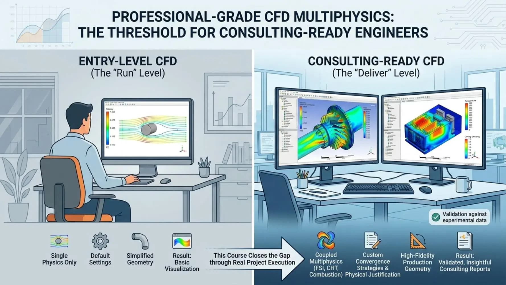
The demand for engineers capable of professional-grade multiphysics simulation spans every major sector: energy systems requiring steam methane reforming (SMR) and plasma gasification analysis, HVAC and electronics industries needing conjugate heat transfer (CHT) and porous media cooling models, and aerospace sectors demanding turbomachinery FSI and combustion CFD at production fidelity. This course closes the gap between expert-level proficiency and professional consulting capability — systematically, through real project execution.
Advanced CFD Solver Competencies & ANSYS Fluent Multiphysics Skills You Will Master
Coupled Physics & Solver Stabilization
Setting up and stabilizing FSI, CHT, reacting flow, and phase change simulations that fail on default solver settings
Writing and applying UDFs and property macros for custom physics and non-standard material behavior
Specialized Solver Methods
Applying dynamic mesh, moving mesh, MRF/SRF, DPM, porous zone, and species transport models to production cases
Configuring VOF two-phase flow, MHD/EHD, PCM solidification/melting, and broadband noise acoustics
Professional Workflow & Deliverables
Managing convergence in transient, two-phase, and high-energy simulations under real project constraints
Translating professional-grade CFD results into engineering conclusions a client would accept
Deploying cases on HPC infrastructure for large-scale transient and multiphysics workloads
Complete Professional CFD Course Modules: 40 Consulting-Grade Multiphysics Projects
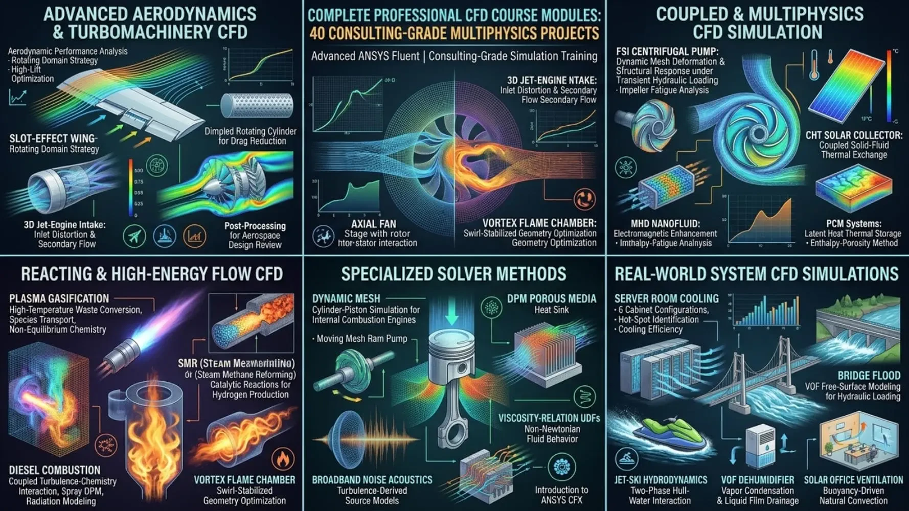
Advanced Aerodynamics & Turbomachinery CFD: Slot-Effect Wing, Axial Fan, Jet-Engine Intake & Dimpled Cylinder
This module addresses the most demanding aerodynamic configurations in professional CFD simulation. Projects include slot-effect wing performance analysis for high-lift device optimization, axial fan-stage aerodynamics with rotor-stator interaction, a dimpled rotating cylinder for drag reduction research, and a 3D jet-engine intake capturing inlet distortion and secondary flow structures. Each case requires advanced turbulence model selection, rotating domain strategy, and post-processing sufficient for aerospace design review — the standard expected in professional aerodynamics consulting.
Coupled & Multiphysics CFD Simulation: FSI Centrifugal Pump, CHT Solar Collector, MHD Nanofluid & PCM Systems
The most technically demanding projects in the course are concentrated here. FSI centrifugal pump simulation couples dynamic mesh deformation with structural response under transient hydraulic loading — directly applicable to pump impeller fatigue analysis and hydraulic seal design. Conjugate heat transfer (CHT) in a flat-plate solar collector resolves coupled solid-fluid thermal exchange for renewable energy system optimization. MHD/EHD nanofluid simulation models electromagnetic enhancement of heat transfer in advanced cooling systems. PCM solar water heater and sandwiched PCM projects apply the enthalpy-porosity method to latent heat thermal storage — critical for building energy systems and off-grid solar applications.
Reacting & High-Energy Flow CFD: Plasma Gasification, SMR, Diesel Combustion & Vortex Flame Chamber
This module covers the most physically complex simulations in the professional CFD domain. Plasma gasification reactor CFD models high-temperature plasma-assisted waste conversion using species transport and non-equilibrium chemistry. Steam methane reforming (SMR) simulation resolves endothermic catalytic reactions within reactor tubes — essential for hydrogen production and petrochemical process design. Diesel gas turbine combustion requires coupled turbulence-chemistry interaction, spray DPM, and radiation modeling at production fidelity. The four-inlet vortex flame chamber project addresses swirl-stabilized combustion geometry optimization — a core competency for gas turbine combustor engineers.
Specialized Solver Methods: Dynamic Mesh, DPM, Porous Media, Acoustics, UDFs & ANSYS CFX
This module builds proficiency in the solver methods that define professional-grade ANSYS Fluent capability. Dynamic mesh cylinder-piston simulation captures volumetric compression and expansion for internal combustion engine analysis. Moving mesh ram pump models hydraulic pressure wave propagation in positive-displacement pumping systems. DPM porous media heat sink simulation resolves particle-laden flow through structured cooling geometries for electronics thermal management. Broadband noise acoustics applies turbulence-derived source models for aeroacoustic prediction in fan and duct systems. Viscosity-relation UDFs enable non-Newtonian fluid behavior for biomedical and polymer processing applications. The module also introduces ANSYS CFX — extending solver competency beyond Fluent for turbomachinery and multiphase applications where CFX offers workflow advantages.
Real-World System CFD Simulations: Server Room Cooling, Bridge Flood, Jet-Ski Hydrodynamics & Solar Ventilation
The final module applies professional CFD simulation to complete engineering systems. Server room cooling with six cabinet configurations resolves airflow distribution, hot-spot identification, and cooling efficiency for data center thermal management. Flood simulation over a bridge uses VOF free-surface modeling to assess hydraulic loading and scour risk under extreme flow conditions. Jet-ski two-phase hydrodynamics captures hull-water interaction and propulsion jet dynamics for marine vehicle design. VOF dehumidifier simulation models vapor condensation and liquid film drainage for HVAC system optimization. Solar office ventilation resolves buoyancy-driven natural convection for passive cooling design — directly applicable to sustainable building engineering.
Professional CFD Engineering Skills & Consulting-Standard Simulation Workflows
Skill Category | Competencies Gained |
|---|---|
Coupled Multiphysics | FSI, CHT, MHD/EHD, PCM phase change, reacting flow stabilization |
Specialized Solver Methods | DPM, VOF, porous media, dynamic/moving mesh, species transport, acoustics |
UDF & Custom Physics | Viscosity-relation UDFs, boundary profile macros, custom material properties |
High-Energy & Reacting Flows | Plasma gasification, SMR, diesel combustion, vortex flame chamber |
Professional Deliverables | Client-grade result interpretation, convergence justification, HPC deployment |
Real-World Industrial Applications of This Professional ANSYS Fluent CFD Training
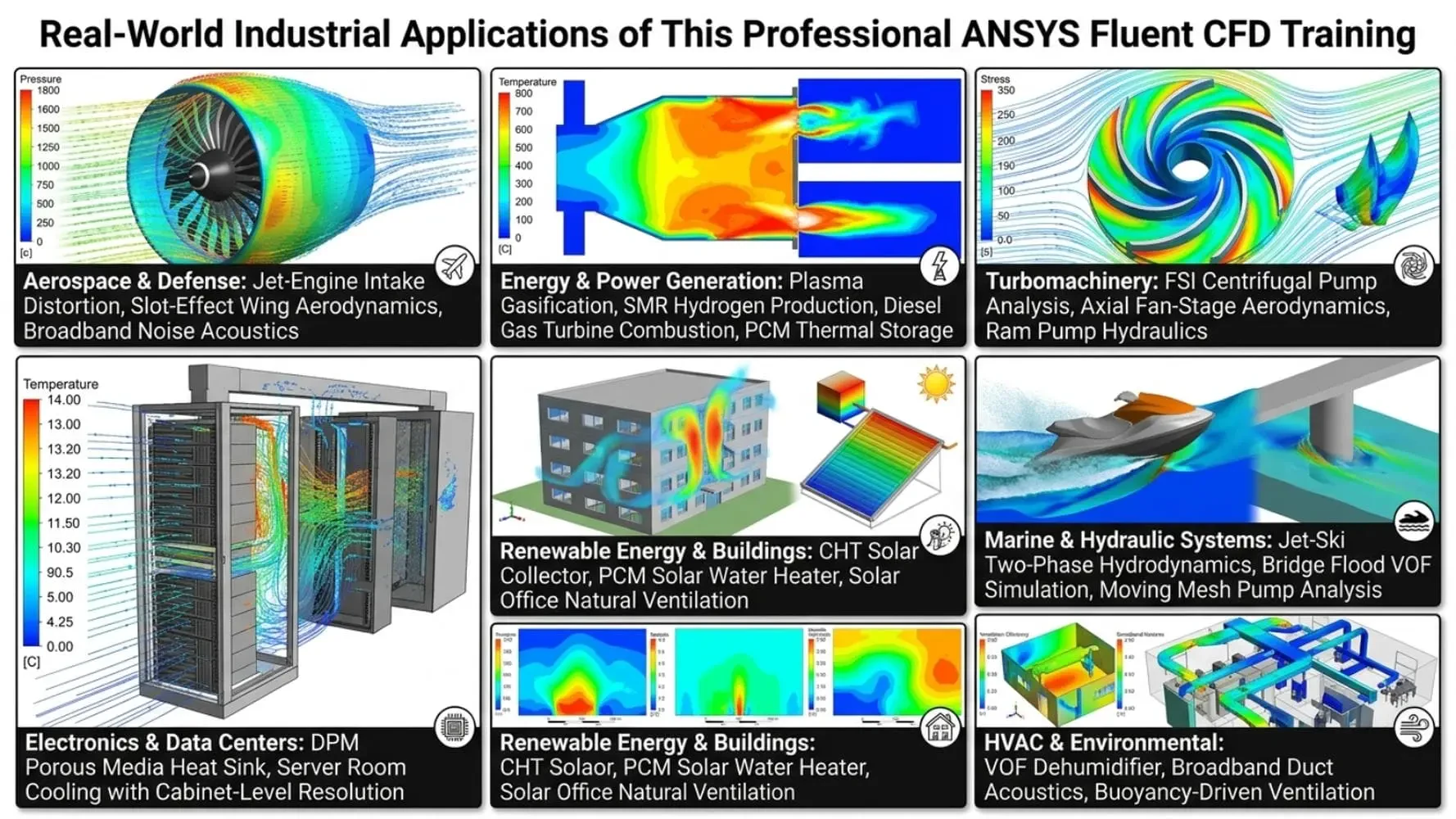
Aerospace & Defense: Jet-engine intake distortion, slot-effect wing aerodynamics, broadband noise acoustics for compliance
Energy & Power Generation: Plasma gasification, SMR hydrogen production, diesel gas turbine combustion, PCM thermal storage
Turbomachinery: FSI centrifugal pump analysis, axial fan-stage aerodynamics, ram pump hydraulics
Electronics & Data Centers: DPM porous media heat sink, server room cooling with cabinet-level resolution
Renewable Energy & Buildings: CHT solar collector, PCM solar water heater, solar office natural ventilation
Marine & Hydraulic Systems: Jet-ski two-phase hydrodynamics, bridge flood VOF simulation, moving mesh pump analysis
HVAC & Environmental: VOF dehumidifier, broadband duct acoustics, buoyancy-driven ventilation
Who Should Enroll in This Professional ANSYS Fluent CFD Simulation Course

CFD Engineers Targeting Consulting Roles: Professionals who need to demonstrate the ability to deliver coupled multiphysics results at client-accepted quality standards
Senior Graduate Researchers & PhD Candidates: Requiring production-fidelity simulations in reacting flows, FSI, or multiphase systems for high-impact publications
Industry Simulation Specialists: Engineers in energy, aerospace, HVAC, or marine sectors who need to expand beyond single-physics workflows into full multiphysics CFD
MR CFD Series Completers: Engineers who have progressed through the Beginner, Intermediate, and Expert ANSYS Fluent courses and are ready for the professional capstone
Prerequisite: Expert-level ANSYS Fluent proficiency including UDF programming, FSI, rotating machinery, combustion, and HPC simulation experience.
Why MR CFD Delivers Unmatched Professional CFD Simulation Training
MR CFD builds its curriculum directly from active consulting practice. Every project in this Professional CFD Course is a real consulting deliverable — not a textbook exercise — which means every modeling decision, convergence strategy, and validation benchmark reflects genuine industrial complexity.
40 Consulting-Grade Projects: Each case mirrors a real MR CFD client deliverable across every major engineering domain
AI-Assisted Simulation Support: One month of Claude AI Premium included for setup checking and post-processing acceleration
Integrated HPC Access: Run heavy transient and multiphysics cases on MR CFD’s dedicated HPC for CFD without hardware constraints
Internship-to-Consulting Pathway: Top graduates access MR CFD’s CFD internship program for live client project experience, with a direct path to CFD consulting engagement
ANSYS Fluent CFD Learning Path: From Beginner to Professional Consulting Standard
Level | Course | Core Focus |
|---|---|---|
Level 1 | Geometry, meshing, boundary conditions, steady-state setup | |
Level 2 | Turbulence modeling, multiphase, heat transfer, transient cases | |
Level 3 | UDFs, FSI, rotating machinery, combustion, HPC workflows | |
Level 4 | This Course — Professional CFD Simulation Course | 40 consulting-grade multiphysics projects across all engineering domains |
Enroll in the Professional CFD Course & Deliver Consulting-Grade Simulation Results
Professional CFD consulting demands more than solver proficiency — it demands the engineering judgment to stabilize coupled simulations, justify model selection, and deliver results that drive real design decisions. This Professional ANSYS Fluent CFD Course by MR CFD provides that capability through 40 real consulting-grade projects spanning every major engineering domain.
Begin your enrollment through MR CFD’s CFD training courses portal and take the definitive step from simulation expert to professional consulting engineer.
This is the top tier of the path, for users stepping up from expert to professional. It is built for people who already handle advanced multiphysics on their own and now want the most demanding, consulting-style projects in the MR CFD library.
The Expert course takes the training wheels off and teaches you to solve coupled, real-world problems. This course goes one level further by collecting the single most advanced project from every engineering field, flow model, and solver module, each one chosen to mirror the kind of work CFD professionals actually get paid to deliver.
The most advanced version of each topic. You work through cases like a plasma gasification reactor, steam methane reforming, a diesel gas turbine combustion chamber, multi-cabinet server room cooling, gas sweetening hydrodynamics, a wind tunnel, a ram pump, and an FSI centrifugal pump. Every project is closer to a real industrial brief than a tutorial.
This is the final step of the path, so it assumes you can already mesh confidently, set up steady and transient cases, and manage advanced physics without hand-holding. If you have finished the Expert course or have equivalent professional experience, you are ready to start here.
ANSYS Fluent plus the geometry and meshing tools used across the lessons (Design Modeler, SpaceClaim, ANSYS Meshing, and Fluent Meshing). As with every course in the path, you bring your own active ANSYS license, student or commercial.
Yes. These are multiphysics-heavy cases that do not fit comfortably on a typical laptop. MR CFD provides HPC infrastructure so you can run cases at this scale without tying up your own machine or waiting days for a result.
That is exactly its purpose. The projects mirror the real consulting work CFD professionals get paid to deliver, and top performers can move into MR CFD's internship program to work on real client projects.
No. Each project is self-contained, so you can go straight to the field, model, or module you need. Since this is the most advanced tier, the earlier courses are the fastest place to fill any gap if a project assumes something you have not covered.